Gallium arsenide (GaAs) consists of larger arsenic atoms (violet) connected to somewhat smaller gallium atoms (salmon pink). Each arsenic atom allows four gallium atoms to covalently attach to it, but those gallium atoms can attach with two other arsenic atoms. This allows the GaAs to have an indefinite molecular size as this pattern repeats, forming what is called a network covalent crystal.
We only consider a single portion of the entire complex called the unit cell, shown in Figure 1. It takes the form of a cubic structure. This unit cell can be placed and attached side by side with other unit cells to complete the crystal.
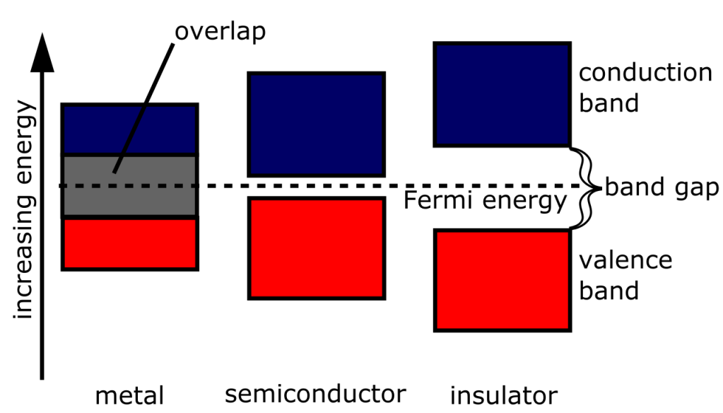
Now, every material varies by its conductivity. Conductivity is determined by how much energy is needed to promote the electron from its bound state to the atoms, called the valence band, to the level in which it can freely move, called the conduction band. The lower the amount of energy is needed to promote the electron – that is, the smaller the “band gap” – the more conductive it is. Conductors thus have a narrow to non-existent band gap, semiconductors are thus characterized by a small band gap, insulators by a large band gap.
Figure 2. Sizes of band gaps. Metals are characterized by overlapping conduction and valence bands.
Synthesis
The most common way of preparing GaAs is through the Birdgman-Stockbarger method. In that method, a crucible containing the polycrystalline material (in this case GaAs) is placed in a tubular furnace where it is heated and made molten. However, down that furnace, there is a temperature gradient – meaning to say, the amount of heat per position inside the tubular furnace varies. In the Bridgman-Stockbarger method, the furnace’s temperature decreases downwards vertically. Thus, the lower regions of the crucible are cooler.
A seed crystal that follows a specific crystal structure is placed at the lowest portion of the crucible. As the crucible is lowered then, the molten gallium and arsenide is cooled and eventually solidifies around the seed, following its structural pattern.
GaAs has become somewhat of a standard material in experimental physics and engineering. Crystals of GaAs also a neat property in which the jiggling of its electrons in the valence band are in sync with the electrons in the conduction band. This property allows it to emit (and absorb) photons with high efficiency.
This makes GaAs useful in constructing near-infrared emitting diodes, which emit photons, and solar cells, which absorb them.
GaAs can also be used as a semiconductor in transistors found in computers, but its low thermal conductivity and high tendency to expand due to heat make it complicated to use. Its low manufacturing cost, however, makes up for such complications.
Computers have always been good in running several calculations at the same time. These have been useful in doing statistical computations or doing simulations. But as the number of calculations increase, the time it takes to collectively do all of them increases – in other words, it’s slower and harder to do large computations.
Understanding natural phenomena isn’t always so straightforward. Sure, we can base it off a set of theorems and laws and predict how, say, a ball of mass m follows a path through space and time. That’s easy, and most of the time we can write down a closed form formula to describe it. But the world isn’t made out of balls of mass m that can understood as a moving point.
When we take a biology class, we’re usually introduced to what is called levels of organization in life. Molecules usually serve as the simplest level, but they themselves are made out of atomic constituents that each have their electrical and chemical properties. As one goes higher in organizational level, we encounter cells which are made out of millions or billions of molecules. And cells, too, organize into tissues, then organs, and whole organisms. Eventually we reach the highest levels of organization which are ecosystems, biomes, and whole biospheres.
A system that has many individual constituents, each following a set of physical laws. But regardless if one has ten, a hundred, or a thousand molecules, they will still each follow those laws collectively. It just gets harder to compute for each of their energies, force terms, positions, and velocities. Thus, they require computer simulations that can do several calculations at the same time. But we said, as the number of calculations increase, it gets harder for the computer to process the data.
Since cells are built of almost too many molecules, it will indeed be hard to simulate an entire organism down to the molecular level. We can indeed simulate how a cell behaves by omitting their molecular constituents and focusing on the bulk of organelles, but that will force us to do numerous approximations that would lead to numerous errors. If we were to do this as accurately as possible, we must minimize the amount of approximations we do, and at best still include individual molecules in the simulation.
Molecular Dynamics
Physicists and chemists have been simulating how a group of molecules behave for a long time. These simulations often include the atomic constituents that build these molecules like lego. Even then, each atom has their own unique electrostatic and mechanical properties.
Molecular dynamics is a method for simulating said molecules. This method takes into account the potential energies and kinetic energies of each atom, which also affects their motion. These atoms can move either by vibrating, moving back and forth, or rotating. The molecule can also be affected by other factors such as the temperature of the environment, which creates random jiggling and fluctuations in movement.
Sometimes, quantum mechanics heavily affects how the body moves and interacts, since at this scale of space the wave functions of electrons around the molecule affects polarity and charge distributions.
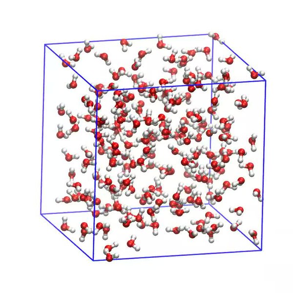
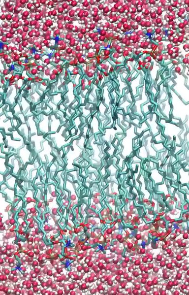
The simulation can also include other molecular bodies, either of the same chemical species or a different one. Below, we can see a simulation of water molecules. But we can also have a simulation of DNA being surrounded by water molecules, or maybe a protein folding. These can show how intermolecular forces affect the physical properties of chemicals. But these models have a catch: they are viewed in isolation, with the only external factor being temperature. In an organism’s cell, the molecules are never isolated from other chemical species.
Computational researchers usually run these simulations in a matter of seconds or a few minutes. But in reality, these happen much, much faster. A 25 second process of a protein folding might actually be representing a 25 nanosecond process. Actually, most molecular dynamics simulations model events that happen in a matter of nano to microseconds. In a way, they recreate what happens in slow-mo.
Now, as previously mentioned, the more calculations needed to be done, the longer it takes to process the data. Since molecular dynamics can involve hundreds of constituent atoms each with their own physical properties, we can expect the computation time take quite a while.
Even though the result of these simulations is a video lasting several seconds or a few minutes, the time it takes to process and produce them actually takes a long time – there are cases when it takes days to calculate all the necessary parameters, and sometimes even days! Supercomputers have thus been designed for the sole purpose of doing molecular dynamics – the IBM Blue Gene, for example, was made to study protein folding. The techniques used in protein folding research using IBM Blue Gene cascaded into other fields and applications that in the end improved our computer technologies.
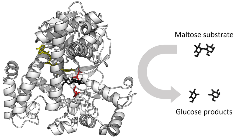
It gets even hairier when we think of simulating reactions such as enzyme catalysis and DNA transcription. Not only do we have a mix of various chemical species physically interacting with one another, but now we also have to model how they change each other chemically – how they displace constituent atoms from their molecules, or how they change the geometry.
The solution to the problem of computational time is to sort of approximate the structure of the chemical species in the reaction. Researchers also omit other factors such as the detailed structure of large molecules. This method is called coarse-graining, wherein the “resolution” of the molecules is lowered, and meanwhile only the bulk effects of certain portions of the molecular structure is considered. The computational processing time is significantly lowered by orders of magnitude through this method. But in exchange, it becomes less accurate as we perform approximations.
Simulating biochemical reactions is especially useful today. Molecular biophysicists use computers to identify compounds that could disrupt the structure of the SARS-CoV-2 proteins, potentially finding a good treatment. It can also aide with finding out how mutations could possibly occur by finding transcription errors in computer simulations. But doing that requires processors from supercomputers already.
Whole Cell
Individual cells themselves are built up of countless biochemical reactions – which as we know now require expensive computational power. Simulating even a single cell now seems impossible. But with coarse-graining, simulating a single cell – with all its biochemical processes such as metabolism – becomes a reality.
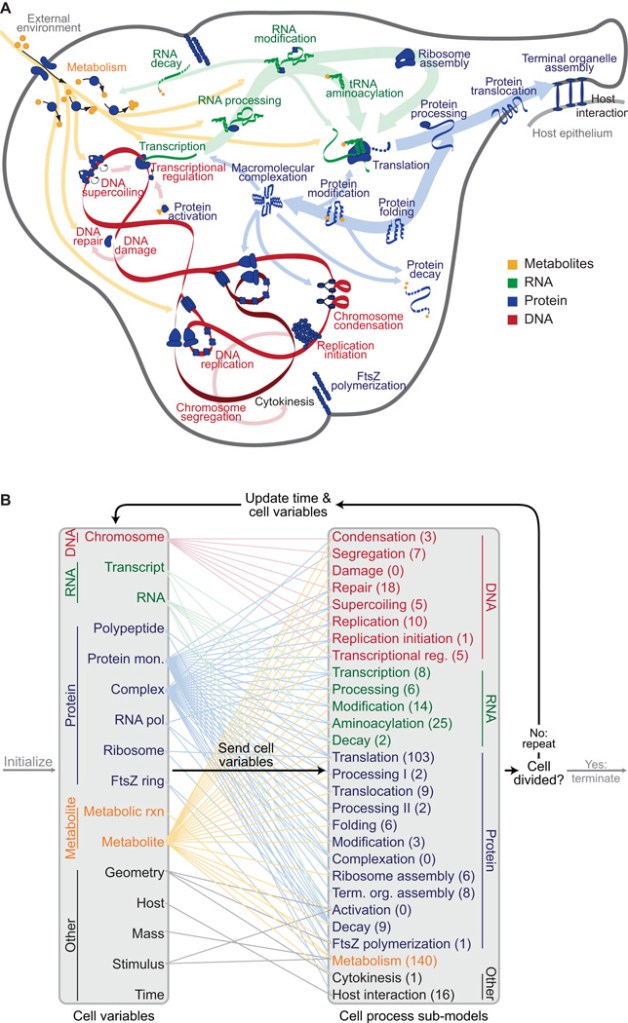
In 2012, Jonathan R. Karr and his colleagues from Stanford, along with scientists from the J. Craig Venter Institute, made a landmark study in biological simulations. In it, they applied what they called a whole-cell computational model to simulate an entire bacterium organisms. Specifically, they were able to simulate the a single Mycoplasma genitalium cell – a pathogen that is transmitted sexually.
They chose this bacteria species specifically because of its extremely small genome – it only contained 525 genes. This meant that it would be easier to identify the individual mechanisms that support it. Based on this genetic sequence only, they were able to predict how the bacterial cell would behave, how it would produce specific compounds, and how it would reproduce.
Using data from 900 different articles and books, they were able to reconstruct the M. genitalium genome with its physical and chemical properties. Each gene was grouped into 28 different cellular processes in which they played a role by producing enzymes and other proteins. These processes involved various biochemical reactions in which these enzymes played a role.
Initially, they simulated each cellular process individually, refining it further. Afterwards, they integrated each cellular process into a single system by determining how their reactants, products, and side products affect each other.
By grouping all the processes together, they were able to simulate the behavior of the entire cell with its individual molecular components solely from this data – from DNA binding protein interactions, as well as metabolism as a cell cycle regulator (the cell cycle is generally the life cycle of the cell that involves reproduction, i.e. cellular division).
They were able to predict how these mechanisms would unfold in detail, thus providing new insight on how to hack them – since Mycoplasma genitalium is a sexually transmitted pathogen, disrupting these processes would be useful for preventing from multiplying and causing disease.
But, as mentioned, the Karr and his colleagues did a form of coarse-graining. Despite simulating the cell down to the molecular level, they did it on a time step of exactly 1 second – as in, they performed it in real time. They did not do a “slow-mo” version of a nanosecond to microsecond event. So there was no protein folding, motion, or geometric reconfiguration of the molecules – instead they only considered the bulk effect, focusing on the input of the cellular process and the output of the cellular process.
Still, what was amazing about this study was their ability to include the molecular components – something that was not previously done. This was by far the best simulation that built a cell from bottom up: based on the genotype (gene sequence) of the bacteria, they were able to predict the characteristics of the organism.
Whole cell modeling, Karr and is colleagues say in their seminal paper, can also be applied to recreating more complex cells such as human cells. This can have profound implications for understanding the dynamics of mutagenic diseases and cancer.
Whole Cell Molecular Dynamics?
As much as possible we would want to avoid coarse-graining if we are to fully simulate the cell down to the molecular level. Molecular dynamics often neglects the presence of other environmental factors other than temperature, while whole cell modeling does not capture the full resolution of what really happens.
There was, in fact, an attempt in 2015 by Feig and his colleagues to bridge this gap. They were able to recreate a whole-cell model for M. genitalium based on genotype just like Karr – the difference was that he started his model with the laws of physics, something done only in molecular dynamics. They included the motion of the proteins and DNA complete with their geometric structure. (You can view the diagrams here.)
It was amazingly complete with all the electrostatic interactions, transport of certain chemical species, and the networks of biochemical reactions all confined within the space of the M. genitalium cytoplasm. It even predicted molecular structures from the gene sequence only.
One can imagine how computationally expensive this was – indeed, they used a large set of powerful supercomputers at the RIKEN Integrated Cluster of Clusters in Japan. One can only imagine how long it took to process such a large amount of data.*
The simulation was also complete with the cellular processes and biochemical reactions present in Karr’s whole cell model. However, as Feig et al. emphasizes, their simulation remained highly speculative due to uncertainties in the complete geometric structure of the M. genitalium genome.
Regardless, this provides a stepping stone for a complete, fully detailed simulation of a general cell. This was a proof of concept that showed a whole cell molecular dynamics simulation was possible. As we continue to understand the cell in its full function and its full resolution , we’d be able to capture in detail the biological processes that drive life.
*I’d admit, I can’t find any sources on how long their computations took
References
Feig M, Harada R, Mori T, Yu I, Takahashi K, Sugita Y. 2015. Complete Atomistic Model of a Bacterial Cytoplasm for Integrating Physics, Biochemistry, and Systems Biology. J Mol Graph Model 58:1-9.
Groenhof G. 2013. Introduction to QM/MM Simulations. In: Monticelli L, Salonen E, editors. Methods in Molecular Biology. New York: Springer Science+Business Media. p. 43-66.
Karr JR, Sanghvi JC, Macklin DN, Gutschow MV, Jacobs JM, Bolival Jr. B, Assad-Garcia N, Glass JI, Covert MW. 2012. A Whole-Cell Computational Model Predicts Phenotype from Genotype. Cell 150(2): 389-401.
Wang JM. 2020. Fast Identification of Possible Drug Treatment of Coronavirus Disease-19 (COVID-19) Through Computational Drug Repurposing Study. J. Chem. Inf. Model. 60(6): 3277-3286.
In the early 1990s, the Philippines – a country known to be one of the greatest victims of deforestation – experienced a sudden slight increase in forest cover. While indeed there have been massive efforts of reforestation in the archipelago, that increase is mainly due to a change in definition of what a forest is. According to the Philippine government’s Forest Management Bureau (FMB) of the Department of Environment and Natural Resources (DENR), a forest is any tree-covered land of an average tree-height of more than 0.5 hectares. This is in accordance with the definition given by the Food and Agriculture Organization (FAO) of the United Nations.
While this definition indeed allows us to protect any tree-covered land to a certain degree, it skews the view on what a forest really is. That could potentially lead to loopholes in restoration, where a mining company after conducting an operation could simply plant trees and claim they have properly reforested the area.
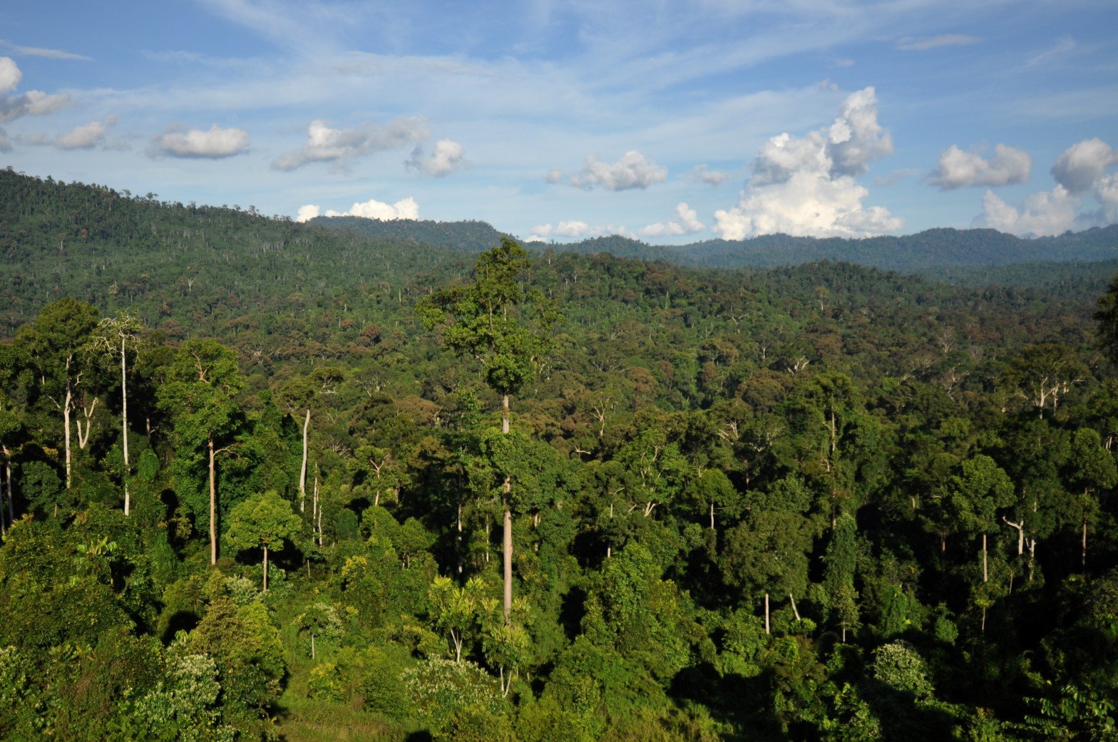
Thus, it is appropriate to discuss what really makes a forest. Here, as we discuss the criteria of a fully functioning forest, we will see that it is much, much more complex that a simple plantation of trees.
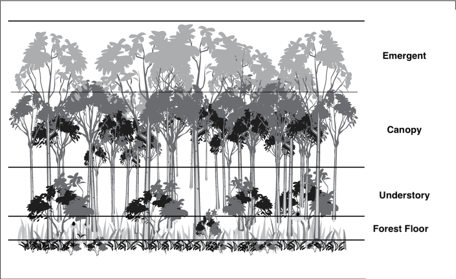
Any forest should indeed have these. Moreover, their presence allows the biome to be divided into four layers: forest floor, understory, canopy, and emergent layer. The forest floor, being the darkest layer, houses homes for insects and other critters. Moss also thrives here among the rocks, providing a large bulk of the oxygen in the entire biome. Much of the nutrients stored in plants are quickly recycled via decay, which are facilitated by detritivores such as fungi and soil bacteria. The nutrients eventually find their way back into the plants. But this section of the biome can already reach a height of 5m. So we can see that the minimum requirement of a forest given by FAO and FMB-DENR is inadequate.
Going a little higher, we reach the understory, which receives little sunshine. Thus, plants here have adapted by evolving broad leaves that have a greater chance of being hit by sunlight for photosynthesis. In tropical rainforests, animals that live here include jaguars, tree frogs, and leopards.
Climbing even higher, the canopy is what we usually see when viewing an expanse of forest. This portion of the forest is usually the most diverse. It can provide a habitat for a vast variety of birds, monkeys, snakes, among others. This is because it is abundant in food, especially when the trees include fruiting trees. Much of the trees here receive the a large portion of sunlight hitting the forest cover.
Lastly, the emergent layer – which can grow indefinitely taller than the canopy – belongs to the tallest of trees that overlook the canopy of the forest. The emergent layer is easily seen as the aggregate of trees that poke out of the canopy, like patrol towers jutting from the ground. The same animals from the canopy can be found here. Many birds of prey such as the Philippine eagle prefer to nest in the emergent layer.
Water Regulation
Water, being crucial in the reactions in photosynthesis, is absorbed by all kinds of plants from the soil. Minerals that are dissolved in it are also taken up by the roots of the plant, thus filtering it. Sources of this liquid include river systems and rain, which also makes the area more humid.
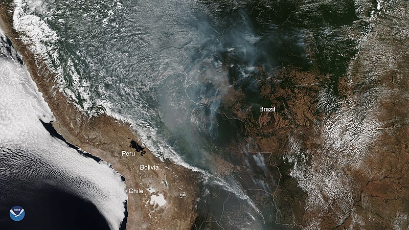
But a large portion of the absorbed water is not used, and manages to escape through the stomata, which are leaf pores that are also responsible for the entry of carbon dioxide for photosynthesis. This process is called transpiration. Thus, the trees themselves also help in making the climate even more humid. This is especially true in tropical rainforests such as the Amazon, where the humidity is so intense that it’s able to form a river of water vapor in the sky in the form large groups dense clouds that travel with the wind.
A denser canopy would also mean less heat and light reaching the forest floor. This leads to better water trapping in both the soil and in the air below the canopy. It would also lead to less transpiration from the trees as the heat stimulates the water to escape, thus allowing the trees to store more of the liquid.
The forest’s water does not only affect the dynamics of the biome itself, but also the surrounding areas. In the previously mentioned Amazon sky river, the water travels through out South America and aides in distributing rainfall throughout the continent. That’s why despite the vastness of the landmass, the only desert lies on a thin section on the Western side of the Andes, opposite the side of the Amazon Basin.
Because of this, the Pantanal – the world’s largest tropical wetland on the southwestern edge of Brazil – formed. The wetland also provides a vast array of species such as capybaras, jaguars, and marsh deers.
Biodiversity
Figure 3. Philippine eagle from a fragmented Philippine rainforest.
Finally, a forest would need to have a relatively higher biodiversity than its surrounding area. This is true for all types of forest, ranging from tropical to boreal. This is because the shelter of the trees creates more habitats and homes for animals and fungi, which then leads to more interaction between them. This interaction triggers evolutionary mechanisms such as mutation and natural selection, thus leading to greater diversity.
However, these mechanisms are more obvious in tropical rainforests. Despite covering only 6% of Earth’s total landmass, they house around 80% of the documented species in the entire world. This intense biodiversity have led to some calling it megadiversity.
Due to deforestation, the menagerie of plants and animals is in danger. Every year, 140,000 sq km of rainforests are destroyed, providing less homes for said species. Even if we continue to reforest areas that have been cleared of trees, it would be difficult to return to its original state of biodiversity. Thus, the better choice is to continue conservation.
And conservation does not necessarily entail the halting of economic activity. In fact, conserving these forests creates a positive impact on economic sustainability. Retaining the biodiversity of these biomes provides a bountiful amount of resources that contribute to medicine, food, rubber, gum, among others. Biodiversity allows a steady chain of supply for these industries that need these resources, as long as the extraction is sustainable and does not disrupt the balance of the ecosystem.
If that balance is disrupted, it would lead to a chain of events that would eventually lead to a loss of species and the forest’s collapse. And if the forests collapse, those vital resources would disappear forever – any plantation of a group of trees won’t mimic the vitality of the original ecosystem.
References
Aron P, Poulsen CJ, Fiorella RP, Matheny AM. 2019. Stable Water Isotopes Reveal Effects of Intermediate Disturbance and Canopy Structure on Forest Water Cycling. JGR Biogeosciences 124(10): 2958-2975.
Anyone who has taken a class from the levels of algebra to vector calculus would be familiar with the concept of the 2D xy-plane or the 3D xyz-space. A point on the xy-plane would be represented as (x,y) where x,y ∈ R. The xy-plane is often denoted as R2 = {(x,y) | x,y ∈ R}. The “2” exponent indicates that it has 2 dimensions and not an exponent.
The notation for 3D space is similar, represented as R3 = {(x,y,z) | x,y,z ∈ R}. We can actually extend this notation for any n-dimensional space as Rn = {(x1, x2,…,xn) | x1, x2,…,xn ∈ R}.
We are now presented with a question: how many points are there in the xy-plane, xyz-space, and further on? In other words, what is the cardinality of R2, R3, …, Rn? Finding this out requires some formal topology, so we will use some intuition.
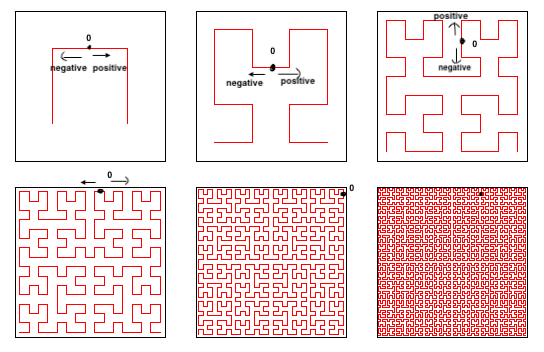
We can actually draw a line throughout the plane that goes on and on, without breaking or stopping. We can assign a point on this line the number 0. Every point before that will be assigned a negative real number, and every point after will be assigned a positive real number.
While we only focused on a Hilbert curve covering a finite space, this can actually go on indefinitely throughout the entire xy-plane. This space-filling curve is called a Hilbert curve, and often comes in handy when assigning a specific point on a plane with a real number. And since we can assign every point with a real number, there is thus a direct correspondence between them, or a bijection. Therefore, the set of points on the plane has the same cardinality as the set of real numbers, or |R| = |R2| = 2ℵ0.
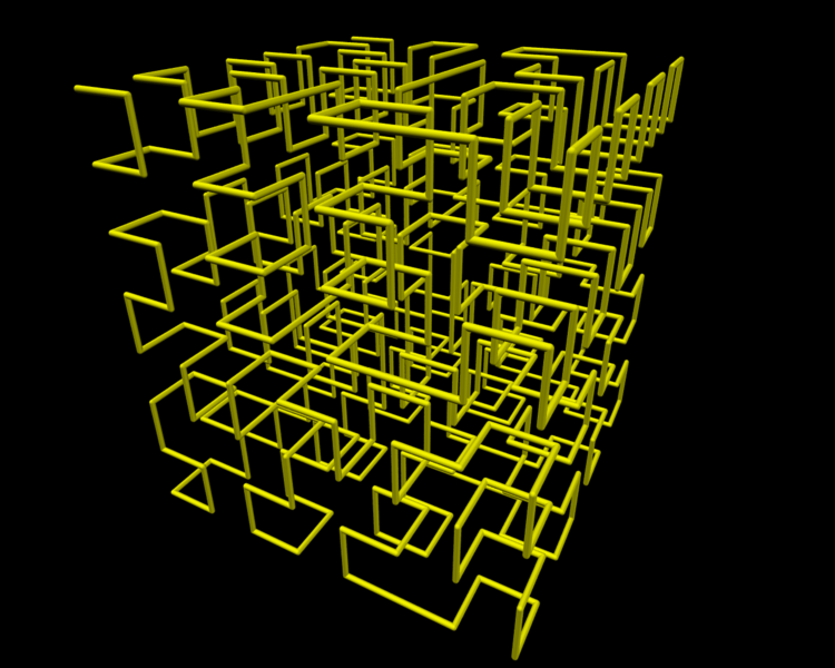
We can do the same for R3, proving |R3| = |R2| = |R| = 2ℵ0.
We can even extend the notion of a Hilbert curve to n-dimensional spaces, thus proving that for any natural number n, |Rn| = |R| = 2ℵ0.
Complex Numbers
In high school, we’re told that √-1 has no solution. Today we know that’s not the case, since we defined √-1 = i, opening up a new set of numbers called the imaginary numbers. The rest of the imaginary numbers are just multiplies of √-1: we multiply any real number with √-1, writing it as bi where b ∈ R.
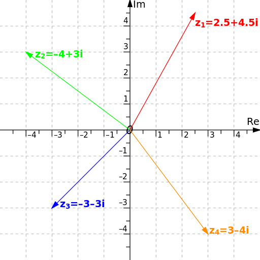
If we add an imaginary number to a real number a, it yields what we call a complex number, which we will call z. We can express z as z = a + bi. The set of complex numbers z = a + bi is also written as C such that C = {a + bi | a,b ∈}. If we multiply z with another complex number such as w = c + di, then zw = (a + bi)(c + di) = ac + (ad+bc)i + (bi)(di). Since i = √-1, i2 = -1. So, zw = ac – bd + (ad + bc)i.
We can see that the set of complex numbers contains the set of real numbers. We can make a complex number have no imaginary component by setting b = 0, allowing i to disappear. Often, the set of complex numbers is represented as a plane.
The main takeaway from here is that any complex number can also be represented as z = (a,b), with a being the real component and b being the imaginary component that is to be multiplied to i. It does not change anything other than the way we represent the complex number. Thus, the set of complex numbers can be expressed as C = {(a,b) | a,b ∈ R}. So if we multiply z = (a,b) with w = (c,d), then zw = (a,b) (c,d) = (ac-bd, ad+ bc). In away, complex numbers are “two-dimensional numbers”.
We can now clearly see that there is a direct correspondence that is bijective between C and R2, and the only difference between the two sets is that you can multiply a point in C with another point in C. This being the case tells us that C has the same cardinality as R2, thus |C| = |R2| = |R| = 2ℵ0.
Beyond
There are actually more numbers beyond the complex numbers. By thinking of complex numbers as two-dimensional numbers, mathematicians have also invented four-dimensional numbers called quaternions, and even eight-dimensional numbers called octonions, and it goes on and on. So far, is are no such thing as a three-dimensional number, or anything in between four and eight, because of the sole reason that it’s hard to craft rules for them.
Those numbers are called hypercomplex numbers. Quaternions would correspond with points in R4 and octonions with points in R8. Since we’ve already established that |Rn| = |R|, we can say that the cardinality of quaternions, octonions, and so on is also 2ℵ0.
So how many numbers are there? There are 2ℵ0 numbers.
References
Rudin W. 1976. Principles of Mathematical Analysis. New York, NY: McGraw-Hill, Inc. 342 p.
Let’s begin with the counting numbers that we were familiar with since preschool. One, two, three, four, five… and so on. We would ask, “what’s the biggest number?”. Someone might have lied to us that it was 100. Obviously, it isn’t – there’s still 101, 102, 103,… and it keeps going.
If we think of any counting number, be it one million, one billion, or the largest counting number we could even type on a word document, there’s always another counting number after that. Just add + 1. So in short, there is no end to the counting numbers. But mathematicians are creative – while we cannot find the largest counting number, they indeed have an answer to the question, how many numbers are there?
And the answer: aleph null, written as ℵ0.
“Wait, what? Is that even a thing?”
Well, according to the current rules we follow in mathematics, this is true. While claiming that the answer is infinity is still correct, this interpretation is more precise since ℵ0 is a type of infinity. As we’ll see in the next sections, there are actually bigger infinities.
In more formal terms, ℵ0 is the cardinality of the set of natural or counting numbers. The cardinality of a set just tells us how many members there are in a mathematical set. For example, the A = {a,b,c,d,e,f} has cardinality |A| = 6.
For numbers, it’s the same. The set S3 = {0,1,2,3} would correspond with |S3| = 4, S4 = {0,1,2,3,4} with |S4| = 5, and set S10 = {0,1,2,…,10} with |S10| = 11. In general, if i is a counting number such that all Sk = {0,1, 2,…, k}, then |Sk| = k + 1.
If we allow i to go on until infinity, eventually we’ll include all counting numbers. Hence, Si would actually be the set of all natural numbers, which we usually call N. Thus, we write aleph null in an equation as |N| = ℵ0..
The concept of aleph null was first crafted in 1874 by the German mathematician Georg Cantor, who is credited as the “father of set theory”. Despite being renowned today, Cantor experienced harsh criticism and backlash from his colleagues due to this extremely counter-intuitive concept. It took years before he was duly credited with his ideas, where in 1904 the Royal Society awarded him with the Sylvester Medal to honor his work.
The Integers
The set of integers Z is the set of natural numbers combined with the negative numbers. This means that Z = {…,-2, -1, 0, 1, 2, … }. We have established that there are ℵ0natural numbers. What about the integers? That is, what happens if we include the negative numbers?
Let’s work on a conjecture: the number of integers equals that of the number of natural numbers. Here’s the proof.
Suppose we have a function f that maps a natural number n to the integers defined as follows
Equation 1
In other words, if n is even, then the functional value is positive. On the other hand, if n is odd, then the functional value is negative. Judging from the values that the function spits out, we can see that for every natural number, there is a corresponding integer and vice versa. In mathematics, we call this a bijective function. And it is easy to believe that if this is the case, then the number of integers is the same as the number of natural numbers. Therefore, there are also ℵ0 integers.
Since there are ℵ0 integers, we can state this as |Z| = |N|. There is a technical term for sets that have the same cardinality as the natural numbers – they are said to be countable sets. It makes sense, since for every member of the set there is a corresponding counting number assigned to it.
The Rational Numbers
The set of rational numbers Q is the set of integers combined with the set of fractions and their negative counterparts. It would be hard to write it down as a list, so we instead we express it as Q = {a/b | a,b ∈ Z}. (| is read as “such that”, ∈ is read as “an element of”).
So how many rational numbers are there? The answer is also ℵ0.
The proof, which was cooked up by Georg Cantor himself, is as strange as the concept of ℵ0 itself. It goes by organizing all the rational numbers into a table: each row represents a numerator, and each column represents the denominator that will divide it.
In effect, we can draw an arrow snaking through each table entry indefinitely, as shown above. The first table entry it hits will be assigned the number 1, then the second the number 2, the third number 3, and so on. We can interpret this as being able to count the rational numbers. So now, we can observe that for every positive rational number, there is a corresponding natural number as it goes on indefinitely.
If we include the negative rational numbers, then we’ll assign them the negative counting numbers such as -1, -2,… Since we’ve already proven that the integers have the same cardinality as the natural numbers, we can therefore say that the cardinality of rational numbers is also ℵ0.
So far, we have proved that the set of rational numbers is also countable since it has the same cardinality as the set of natural numbers. If we were to write an equality representing the cardinality of the set of rational numbers Q, then it would be stated as |Q| = |N| = ℵ0. We can already see that |Q| = |Z| as well from the previous section.
The Real Numbers
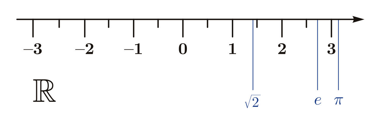
The set of integers contain the set of natural numbers, and the set of rational numbers contain the set of integers. Similarly, the set of real numbers contain the set of rational numbers, plus some additional elements called the irrational numbers. This includes the numbers π, e, √2, and numbers with never ending decimals that do not have a predictable pattern, such as 5.123899817283197… The set of real is usually represented as R.
Do the real numbers have the same cardinality as the natural numbers – that is, are they countable? The answer to this requires a rather formal proof, so this will require a lot of focus.
We allow a set A to be a countable set (|A| = |N|) containing never ending decimals with no predictable pattern. We list them down on the table below:
1
1.7219804378291740192…
2
2.1245156325342523454…
3
7.1239190283901293810…
4
6.1231262812934810294…
5
0.1239809182371827381…
6
4.1273891273891239801…
7
0.6127836816278317816…
8
5.1329815012903813191…
9
3.6294038502858290385…
10
9.1239081293081391238…
Table 1. A list of numbers with decimals with no predictable pattern.
For every nth number (assigned in the left column), the nth digit is colored red (with the number before the decimal being the first digit). We can write a number whose nth digit always differs from the nth digit from the nth number: 2.235094767… This means that this number differs from each member of A by at least one digit – therefore, this number does not belong to A.
Since we can replace the elements of A with any other decimal, this proves that every countable subset A of R is a proper subset – meaning, that there’s a number in R that’s not in A. This is subtle, but very crucial.
This implies that if R was countable, then it would also be a proper subset – meaning that there’s a number in R that’s also not in R, which does not make any sense. Thus, the set of real numbers R is uncountable.
So what does this tell us? Since the set of real numbers is uncountable, it follows that its cardinality is not the same as the set of natural numbers, ultimately meaning that the cardinality of R is not equal to ℵ0. We write this as |R| ≠ ℵ0.
This begs the question – how do we represent |R|?
Intervals
We can think of a subset J of R of all the numbers between 0 and 1. We can prove that |J| = |R| by thinking of a function that assigns every real number with a number between 0 and 1, just like how we proved that |Z| = |N|. Any function that does the job will do, but the simplest one is presented below
Equation 2.
With x being a real number. So since we can assign all real numbers with a specific number between 0 and 1, we can say that |J| = |R|. This result will prove useful in the next section.
The Power of Power Sets
Let H be a subset of natural numbers, say G = {1,2} so |G| = 2. Then its power set of G, P(G), is the set of subsets of G. We can actually list down the power set’s elements: P(G) = {{},{1},{2},{1,2}}. We write the empty set, which is the set that does not contain any elements at all, as { }.
We can notice that the cardinality of P(G) is |P(G)| = 4 = 2|G| = 22. If we choose another set H = {1,2,3} with |H| = 3, then P(H) = {{},{1},{2},{3},{1,2},{1,3},{2,3},{1,2,3}}. So, |P(H)| = 8 = 23 = 2|H|. This trend actually continues for any set. So we can actually say that any set X, the cardinality of its power set P(X) is |P(X)| = 2|X|.
So what if we consider the power set of the natural numbers P(N), such that |P(N)| = 2|N| = 2ℵ0? It will be hard to list them down, but it would look something like {{},{0},{1},{2},….,{0,1},{0,2},…,{1,1},{1,2},…{1,2,…}}. Now here comes another crucial part, in which understanding it will require a lot of focus again.
We can think of a number between 0 and 1 whose decimal digits have the same order as a subset of N, which is always a member of P(N). Examples are shown below.
{1,2,3,4,5,6,7}
0.1234567
{2,3,4,5,6,7,8}
0.2345678
{1,2,3,4,5,6,7,…}
0.1234567…
{5,6,7,8,9}
0.56789
{11,12,13,14,15}
0.1112131415
{11,12,13}
0.111213
{3,4,5,6,7,8,…}
0.345678…
{0,1,2,3,4,5}
0.12345
{0,1,2}
0.12
{8,9,10,11}
0.891011
Table 2. Assigning a number between 0 and 1 to a member of P(N).
Since we can assign a number between 0 and 1 with a corresponding member of P(N), that is, a subset of N. Thus, since in the previous section J represents the numbers between 0 and 1, |P(N)| = |J| = |R|. Thus, |P(N)| = 2ℵ0 = |R|.
We find that the cardinality of the real numbers is 2ℵ0, which is obviously bigger than ℵ0. This goes to show that there are infinites bigger than other infinites. We can actually stop here and say that there are 2ℵ0 numbers, since the real numbers are the only ones we use in measuring things such as length, mass, time, etc. But we can actually go even further.
A simple assembly of atoms: two hydrogens, one oxygen. Its formal chemical name is dihydrogen monoxide (H2O), but of course we never call it that — we call it water.
Despite being so simple, it’s amazing to see how water’s simple structure and arrangement of atoms have led to consequences such as weather, climate, habitable planets, and eventually, life. Here we explore how this molecule has been profound in almost every aspect in science, and even in the understanding of human civilization.
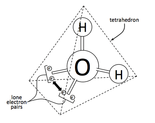
The geometry of a water molecule is actually a tetrahedron, with two hydrogen atoms poking out like the handles of a bicycle, and two lone pairs of electrons in similar arrangement. Here, it is clear how oxygen tends to grab the electrons more, especially since hydrogen still manages to give up its single electron for covalent bonding. Oxygen is said to be more electronegative than hydrogen.
Since the electrons tend to condense around the oxygen atom more, that side has a more negative partial charge. This imbalance of charge results in what is called polarity. This polarity allows the water molecule to electrostatically interact more with other molecules with polarity, both water and those other than water. Thus, water can freely mix with other similar substances: like dissolves like.
But when water molecules interact with each other, the attractive force known as hydrogen bonding is so intense that separating them requires a lot of energy. That’s why drinking even just a quarter of a liter brings a feeling of coolness, and also why bathing seems to dispel the summer warmth – water absorbs so much heat. Thermodynamically speaking, they have a high heat capacity.
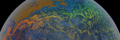
Its effects can be seen at a planetary scale. Ocean currents dissipate heat throughout the globe, creating more tolerable climates both at the warmer areas of the world and in the colder. Europe would be a cold wasteland if it weren’t for the Atlantic currents such as the Gulf Stream.
In its liquid and gas state, water is used as a reference model for fluid mechanics, being the substance that’s practically everywhere on the surface of the Earth.
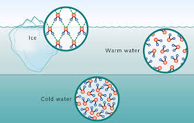
Its geometry also has effects on how it transitions from one phase of matter to the other. At room temperature (298 K or 25 deg C), scientists often set water’s density to 1.00 g/cm3 (as per Table 1), hence being the reference value for all densities of substances. This is because it’s so abundant – even the air carries water vapor. But at lower temperatures, things start to get weird: water’s density continues to increase as it is cooled, until it reaches 4 deg C – where it reaches its maximum density. Colder than that, it starts to arrange itself into ice – which, because of its crystal structure, creates spaces in between molecules that result into lower mass per volume. This actually explains why icebergs float, and why its liquid states exist below the surface of frozen lakes, ponds, and rivers.
Earth is in the Goldilocks zone of the Solar system – an area around a star (in this case the Sun) that’s not too hot for water to evaporate and not too cold for water to freeze over. Its conditions allow for mostly liquid water to thrive, with some areas that are frozen, serving as a reservoir.
There are actually two theories on the origin of water: one is that they came from external sources such as comets (which are basically dirty snowballs in space), and the other is that they were outgassed from the depths of the primordial Earth via volcanic eruptions.
If the external source theory were true, then the ratios of hydrogen isotopes on modern day comets and our oceans would be the same. Hydrogen, being an integral component of water, can come in the form of protium (one proton, one electron), deuterium (one proton, one electron, one neutron), and tritium (one proton, one electron, two neutrons). When geologists measured the ratio of deuterium to protium on the comets Halley, Hyutake, Hale-Bopp, and 67P/Churyumov-Gerasimenko, they found that it was twice that of Earth’s waters. Thus, the external source theory is implausible.
The volcanic outgassing theory, then, is more plausible. Today, volcanoes do expel roughly the same gases as those outgassed in Earth’s early history, but not on the same scale. The intense heat and fluid-like motions of the mantle billions of years ago would have resulted in a massive escape of gases dissolved in the molten liquid, water vapor included. As the Earth cooled, the water would condense and then form our seas and oceans.
The formation of vast swaths of liquid water on Earth would prove essential for the development of the lush world we know today. The surface of the globe today is 75% water. Compared to planets like Mars or moons like Europa – which both have water mostly in the form of ice – our world’s oceans harbor an uncountable number of living things. This is all because water serves as a perfect medium for the development of complex objects such as life.
Birth of Life
The life-giving properties of water is not an exaggeration: it serves as a medium that carries and circulates polar biomolecules and minerals throughout the body. This same circulation of water also regulates the organism’s internal temperature, allowing life to function at usually 37 deg C, where most biological compounds are at its most functional and active. But other than being a medium for life, it’s also possibly the reason why life began in the first place.
Many people often wonder how such a complex system such as life emerged. Some even claim that this seemingly high order of organization violates the second law of thermodynamics, which roughly states that the disorder of an isolated system must always increase. That can be partially explained by arguing that living things are open systems and not isolated ones since they regularly excrete waste and take in energy. While this is true, it’s not the full picture. Actually, the very biomolecules of life – proteins, DNA, phospholipids – can increase the system’s entropy as they organize. We just need to add water.
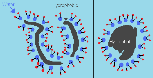
The long string of amino acids known as proteins have certain portions that are hydrophobic – or water-hating – and regions that are hydrophilic – or water-loving. In other words, one side repels water molecules, and the other attracts them. Alone, proteins cannot fold since certain regions attract and repel each other, thus preventing it from conforming to an ordered geometry. But the presence of water sort of forces them to do so without violating any physical laws.
When water molecules are exposed to the hydrophobic portions of the protein, they tend to arrange themselves since their movement is restricted. Thus, the entropy of these molecules decrease. But when they are exposed to the hydrophilic portions, their interactions allow them to move freely, as if it was business as usual since the polarity of the hydrophilic portions resemble that of water. Thus, the entropy increases. In fact, this increase overrides the decrease in entropy when the protein starts rearranging itself. In other words, the net entropy increases.
The process and explanation is the same with DNA molecules when they fold. It also happens with plasma membranes which are composed of phospholipid molecules with hydrophobic lipid tails and hydrophilic phosphate heads. Tucking the hydrophobic tails away from the water to allow the surrounding molecules to move freely. The phospholipid molecules then array themselves to create a sheet, forming a barrier against the water medium.
As these biomolecules are able to assemble into complex structures in the presence of water, some of their forms tend to be sturdier in the presence of external factors such as ultraviolet radiation, oxidative chemicals, and reductive chemicals. Those biomolecule forms thus survive more, allowing them to mutate to even sturdier forms that are more complex. Eventually, these molecules aggregate with each other to give birth to living things.
It’s then no wonder why humid and tropical places such as the Amazon and the Coral Triangle harbor such intense biodiversity. Life relies on water so much that the beginning of our societies rests on the presence of fresh water around lakes and rivers.
We Go Where Water Goes
Even in the driests of deserts, if a river flows, a small sliver of land would become wet and fertilized with the minerals that come with the flowing water. We humans would then cluster around these rivers, first to build agricultural communities on the fertile land. As population grows due to the abundance of food, villages, towns, cities, and eventually empires appear. The first foundation of civilization was the presence of water.
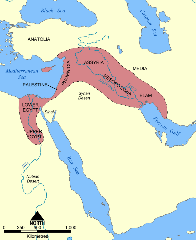
The Indus River provided the ancient Indians with an oasis in the midst of dry land. The Tigris and Euphrates rivers formed a fertile crescent in the middle of a desert, allowing the Babylonian and Sumerian Empires to form, establishing sophisticated cities in the Middle East. The Yellow River in continental East Asia allowed the Chinese Empire to grow. The Nile River gave sustenance to the Egyptians who would build the Sphinx and the Pyramids.
Even in modern society, the presence of clean water can be a determinant of how developed the area is – either it is underdeveloped, or its rapid industrialization has led to sewage problems. And this is of course still an issue, as places such as rural Africa lack filtered water. Meanwhile, dense urban cities such as those in the United States, India, and China have challenges with water pollution, and authorities are looking for new innovations in order to solve this.
As we humans look for planets to expand to, we actively search for ones that harbor water, preferably liquid water. That’s why astronomers are always excited to find worlds in the Goldilocks zone. While we have found worlds like that – some even with liquid water – we still cannot determine if its conditions for habitability suit humans.
Our strongest candidates today in our Solar system remain to be Mars and the Galilean moon of Europa, despite not being in the Goldilocks zone. Astrobiologists are also speculating that certain conditions such as underground volcanic activity could warm subterranean lake chambers or underground oceans, providing conditions for life to develop.
Water is ubiquitous – and while many of those with proper access to clean water take it for granted, its presence has driven the development of both life and society. Its simple geometry and composition has had far reaching consequences, and if it were different, we probably would not even exist. The next time you run a tap to wash your hands or brush your teeth, think of how this magical substance has led to where human civilization is now.
References
Khan MY. 1985. On the Importance of Entropy to Living Systems. Biochemical Education 13(2): 68-69.
In the laboratory, helium hydride is produced by bombarding a low pressure hydrogen-helium mixture with electrons. Although helium hydride has been detected in space, not much is known about its natural formation.
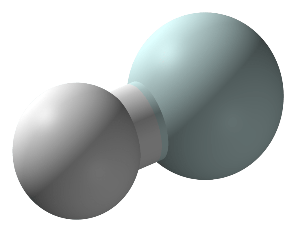
The structure is quite simple, since it is a linear molecule of two atoms. It consists of a neutral helium atom at one end and a positively charged hydrogen atom in the other. Having only two electrons, it’s as if the helium atom is donating its electron to the hydrogen atom in order to neutralize it.
History and Trivia
Scientists first knew about helium hydride when it was synthesized in a laboratory in 1925 by T.R. Hogness and E.G. Lunn using the method mentioned above. Because it contains a positively charged hydrogen atom, they hypothesized that it was a strong acid: it would donate the hydrogen atom to most substances it comes in contact with. However, its physical and chemical properties are not yet well studied, so this is still yet to be proven.
But the existence of helium hydride dates back all the way to 380,000 years after the Big Bang. In fact, some scientists even think that it’s the first compound that ever existed. Since helium and hydrogen were one of the first elements to form, the early conditions of the Universe allowed helium to collide with a proton (which is the same thing as a positively charged hydrogen atom), hence forming helium hydride. This reaction releases energy in the form of photons.
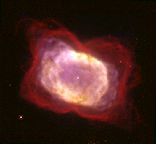
Helium hydride is thought to hide in nebulae and early regions of our galaxy, floating around while remaining intact. This was conjectured in the 1970s, but was only confirmed recently in 2019 by Rolf Güsten and his colleagues from the Max Planck Institute for Radio Astronomy.
Güsten and his colleagues pointed an airplane-based telescope at the planetary nebula NGC 7027. Using tetrahertz spectroscopy, they were able to detect the spectrum of helium hydride, finally confirming the hypothesis that remained unanswered for nearly 50 years. As of now, more research needs to be done on helium hydride in order to determine its other properties, such as acidity and reactivity.
Güsten R, Wiesemeyer H, Neufeld D, Menten KM, Graf UU, Jacobs K, Klein B, Ricken O, Risacher C, Stutzki J. 2019. Astrophysical detection of the helium hydride ion HeH+. Nature 568(7752): 357-359.
Hogness TR, Lunn EG. 1925. The Ionization of Hydrogen by Electron Impact as Interpreted by Positive Ray Analysis. Phys. Rev. 26(1): 44-55.
Life has underlying physics behind it — and that’s a well known fact. After all, everything is physics. But most of the time, physics is concerned with objects almost totally unrelated to biology — things smaller than cells such as atoms and photons, or things bigger than biospheres such as galaxies and stars.
But there’s a field of study called biophysics. While not well represented in popular science media, biophysics is very much alive in terms of research. Understanding the physics of life is not very obvious due to its extreme complexity, but the recent decades have seen progress in connecting the concepts of energy and entropy to things like proteins and evolution.
We’ll quickly tour how physics is applied to biology, down from the level of molecules up to the level of populations. Brace yourselves, since we will quickly jump from one topic to the next.
A Macroscopic Understanding
Prior to the advent of sophisticated laboratory equipment which allowed us to peer into the submicroscopic world, the application of physics to biology was limited to the level of organs and cells.
Bones and muscles are responsible for generating forces and torques that result in displacement. This is generally well understood in the context of classical dynamics and statics. Despite relying on centuries-old theories, biomechanics — which is the field that studies these — is still very much alive in research today. How the bones and muscles are arranged, how they affect one another, and how they are stimulated by the nervous system is quite complex and thus often rely on computer simulations to understand them.
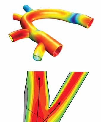
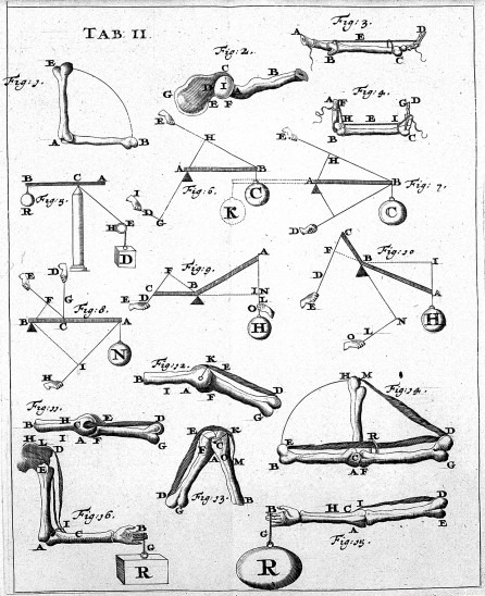
Figure 1. Left to right: (a) Blood flow modeling in blood vessels, (b) the forces in bones from De Motu Animalium by Giovanni Borelli.
Biomechanics is also important in understanding blood flow through fluid mechanics, as well as studying how the gases found in the same blood diffuse across membranes. These models mostly work on the macroscopic level.
The physical understanding of life on this level plays an essential role in medical research. Developing prosthetics would require a solid foundation in biomechanics, as they would need to mimic the movement of the same bones and muscles. The fluid nature of blood is pertinent to the understanding of hypertension and blood clots. But a huge bulk of the physics research today in biology talks about objects smaller than even the cell.
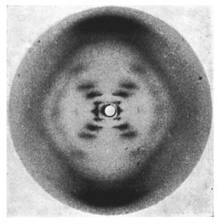
With the elucidation of the structure of DNA by Franklin, Watson, and Crick using X-ray crystallography, the physico-chemical nature of life was beginning to be more and more apparent. And in recent years, physicists, biologists, chemists, and even mathematicians have encountered a fundamental problem in one of the main molecules of life: proteins.
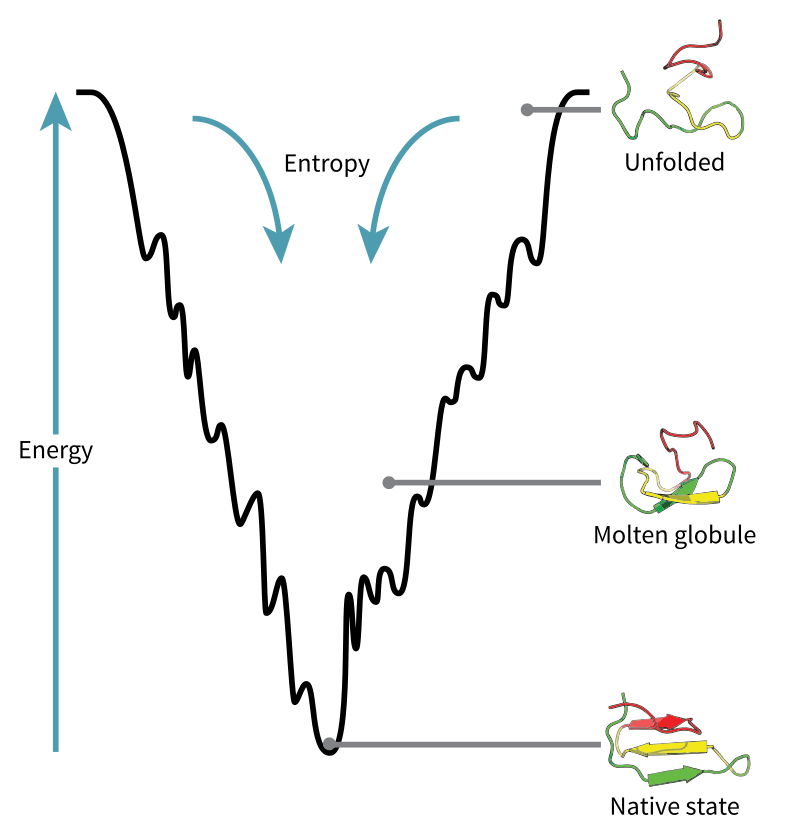
Proteins are an assembly of various units of amino acids, which themselves have different properties. Thus, when these amino acids are strung along together into a chain, some of the units attract each other, and others repel, allowing the chain to fold and crumple to conform to a specific geometry. This is called protein folding. Now, as simple as it may seem, it’s anything but that.
Many factors fall into obtaining the shape of a protein. For one, there are external factors. While temperature of the surrounding environment affects the energy of folding, the medium (usually water) also exerts intermolecular forces on the protein subunits which in turn affect the folding process. There are internal factors as well: the amino acid units themselves can repel and attract other amino acids units in the protein. One can only crunch a limited amount of data to obtain at least an approximate view of the resulting protein shape using computer simulations — which, by the way, takes a great deal of time to process.
Because of the presence of atomic interactions, some quantum mechanics computations are involved in the computation. But overall, most models of protein folding use statistical mechanics to study the relationships between the many particles involved in the system. In a statistical mechanical model, the properties of the many components involved are understood in terms of the probable energies and entropies – hence, statistical.
The concept of protein folding has profound implications in developing medicines, where certain proteins are drug targets which the pharmaceutical acts on. Protein misfolding is also relevant in neurodegenerative diseases, since misfolding leads to malfunction of certain biological processes. For further discussion, you may check out Reynaud’s article on Nature.
Molecular biophysics also involves the imaging and elucidation of the structure of various biomolecules including both proteins and DNA. Currently, techniques involved in such imaging are cryo-electron microscopy, X-ray crystallography, and optical tweezers.
This field of biophysics is especially important in relation to COVID-19 pandemic. Recognizing the structure of the spike proteins that coat the SARS-CoV-2 virus will aid in the invention of vaccines and drugs for treatment. However, this method of course applies to any kind of virus.
Now we can clearly see that biophysics integrates concepts from classical physics and modern physics. But the application of these principles is not always obvious when one considers higher levels of organization. At the level of proteins already, scientists stumble upon problems that are nonlinear. As one delves deep into the field of biophysics, a common theme could be observed: complexity.
Increasing Complexity
As complexity increases, certain minute details are intentionally left out. In a complex system, tracking the behavior of every component would be onerous.
Modeling the behavior of complex systems would rely on recognizing the pattern of their behavior. This contrasts with predicting phenomenon by deriving equations from a prescribed set of principles. Oftentimes when the patterns are recognized, a computer simulation would run to determine how the complex system changes.
Actually, a lot of research in biophysics involves modeling biological phenomena using an analogy from simpler physical phenomena, which can be described mathematically. This way, complexity of the system is somewhat simplified.
For example, birds in a flock might be viewed as similar to moving fluid particles. Or ants in a colony can be modelled as cellular automata, in which the level of order and disorder of movement can be understood in terms of entropy.
Figure 5. (a) Birds in a flock, (b) ants in a foraging trail
Clearly, the smaller details would not be relevant. How the neurons fire to recognize a path wouldn’t be important in determining the patterns of its work. The mechanism of the bird flapping its wings wouldn’t be crucial in recognizing flight direction patterns. Nor would the folding of the protein in SARS-CoV-2 be important in predicting how the COVID-19 would spread from location to location.
Understanding how life itself began is a matter of examining a complex system of interacting molecules. Since biomolecules such as proteins themselves are already complex, what more for the emergence of life?
Life Itself Emerges
One of the criteria for things to be considered life is that they reproduce. Other scientists might call this self-replication, because, well, they produce copies of themselves by themselves. Interestingly, this means that life begins as an order out of disorder. This sounds like it violates the second law of thermodynamics, which roughly states that the disorder of the universe must increase.
In 2013, Jeremy England published a paper that asserts that this is not the case. Actually, he proved mathematically that self-replication is bound to happen. Life would have begun as a set of molecules that was able to replicate itself. The molecule will often restructure itself to dissipate energy, hence following the second law of thermodynamics. And most of the time, that restructuring will reduce its chance of being degraded, thus becoming more abundant. This agrees with Darwin’s principle of natural selection.
Eventually, those molecules — nucleic acids such as RNA and DNA, and proteins — would assemble with each other to form cells and organelles, thus forming the first unicellular organisms. The rest is history after that.
England’s theory is yet to be proven, but its use of physical principles with its underlying mathematical rigor makes it hard to doubt. An experimental proof of this theory would make the physical understanding of life less elusive.
In conclusion, life is extremely complex, from the smallest protein that folds to the behaviors of populations of organisms. But biophysicists are challenged with breaking down this complexity in order to predict and understand its behavior. And while the challenge is difficult, the latter half of the 20th century and the recent years of the 21st have seen great strides. And with finding out how life began, we can finally connect the pieces in the physics of life.
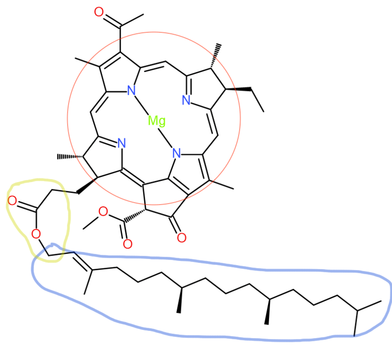
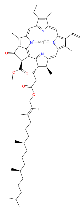
The “head” portion (encircled in red) of the bacteriochlorophyll consists of a partially hydrogenated porphyrin ring known as chlorin. It contains a central magnesium atom. Meanwhile, the “tail” portion (encircled in blue) is a hydrocarbon chain, connecting to the head by an ester (encircled in yellow).
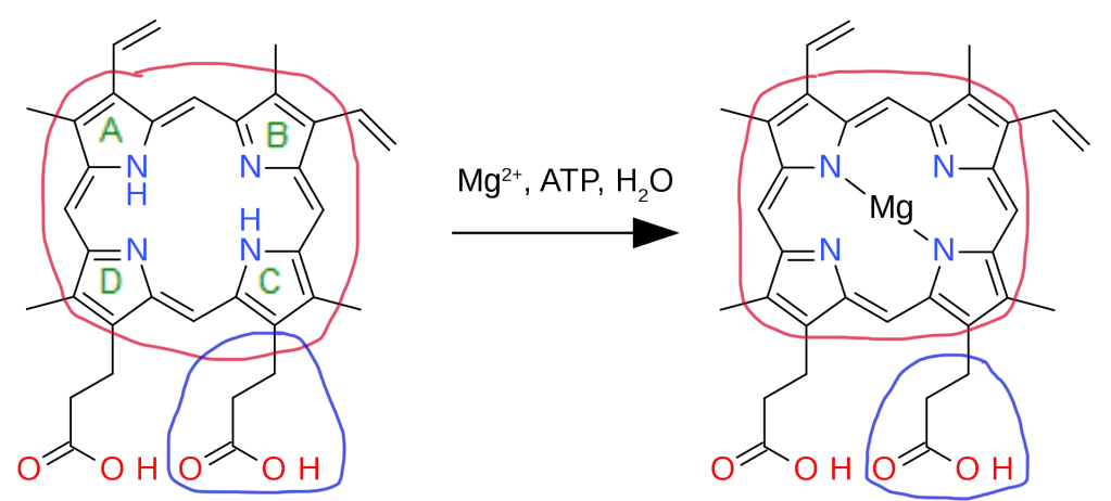
Bacteriochlorophylls, as its name suggests, are a type of chlorophyll produced by photosynthetic bacteria. The biosynthesis of bacteriochlorophyll a in particular begins with protoporphyrin IX previously synthesized from glutamyl tRNA. Magnesium is first inserted into protoporphyrin IX (encircled red) with the help of ATP in an aqueous medium. This reaction is catalyzed by the enzyme magnesium chelatase.
Focus on the group of atoms on the lower right attached to the main ring, encircled blue (a carboxylic acid). The hydrogen is removed and a methyl chain is added (CH3). This reaction is aided by the enzyme Magnesium protoporphyrin IX methyltransferase.
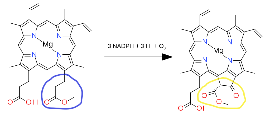
Keep your attention on the previously modified group of atoms that are attached to the main ring, encircled blue (now an ester). With the help of three electron donors known as nicotinamide adenine dinucleotide phosphate (NADPH), the enzyme Magnesium-protoporphyrin IX monomethyl ester (oxidative) cyclase adds three H+ ions and an O2 molecule. This greatly alters the structure of the ester branch into a group of atoms with a very different geometry, but it continues to cling on to the porphyrin ring (encircled yellow). The resulting product is protochlorophyllide.
The chlorin is then converted into a chlorophyllide a using the enzyme protochlorophyllide reductase. The reaction still requires the same electron donor NADPH. As the electron is donated to an H+ ion to become a hydrogen atom, this same neutral hydrogen atom is added to the molecule to slightly change its structure.
Finally, on the carboxylic acid group on the chlorophyllide a product encircled in green, the hydrocarbon chain is attached by a series of reactions using ATP, water, and H+ ions carried out by a series of enzymes. The end product is bacteriochlorophyll a, as depicted in Fig. 1. For bacteriochlorophyll b-g, the process is similar, only with slight modifications involving how specific enzymes modify the structure of the molecule.
Uses
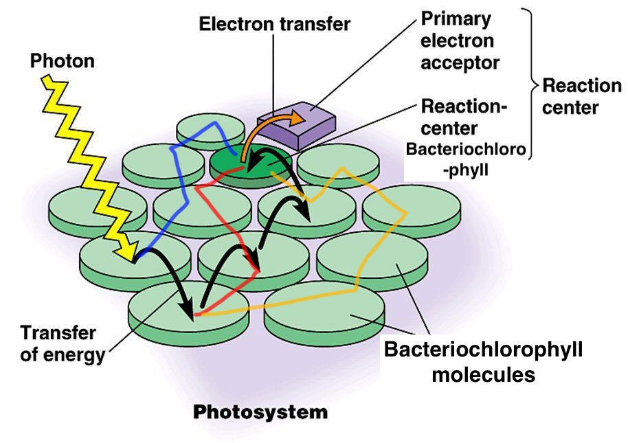
Bacteria such as Chlorobium tepidumuse bacteriochlorophyll in order to harvest light energy in the form of photons for photosynthesis. Similar to the process found in non-bacterial chlorophylls, the incoming energy from the photons liberates electrons from the molecule. This allows the electrons to be bounced and passed from one bacteriochlorophyll to another until it finally finds its destination, the reaction center.
Many bacteria use bacteriochlorophyll in anoxygenic photosynthesis, which produces not oxygen (O2), but sulfur (S). It also requires hydrosulfuric acid (H2S) as a reactant rather than water (H2O).
Trivia
Bacteriochlorophyll are found in Fenna-Matthews-Olson (FMO) complexes, wrapped around by a protein scaffold. These FMO complexes, with the help of the bacteriochlorophylls, are theorized to use quantum light harvesting in order to efficiently use the energy obtained from incoming photons.
Because the electron needs to jump from bacteriochlorophyll to bacteriochlorophyll before it reaches the reaction center, the electron can eventually get lost along with the energy it carries with it. But experiments show that photosynthesis happens at nearly 100% efficiency.
According to quantum mechanics, the electron is both a particle and a wave. Thus, due to its wave-like properties, it can be in several places at once as it is spread out across the material – a superposition of locations. But being a particle, one can only observe it to be in one place. Hence, the wave is interpreted as a sort of probability distribution of where the particle might be.
This can also be interpreted as the electron traveling an infinite number of possible paths at the same time as it covers all locations. Thus, according Engel (2011), since it takes all possible paths at the same time, it can find its destination without losing any energy.
References
Urry LA, Cain ML, Minorsky PV, Wasserman SA, Reece JB. 2017. Campbell Biology 11th Edition. New York City (NY): Pearson Education. 1284 p.
Engel GS. 2011. Quantum coherence in photosynthesis. Procedia Chemistry 3 (2011): 222-231.
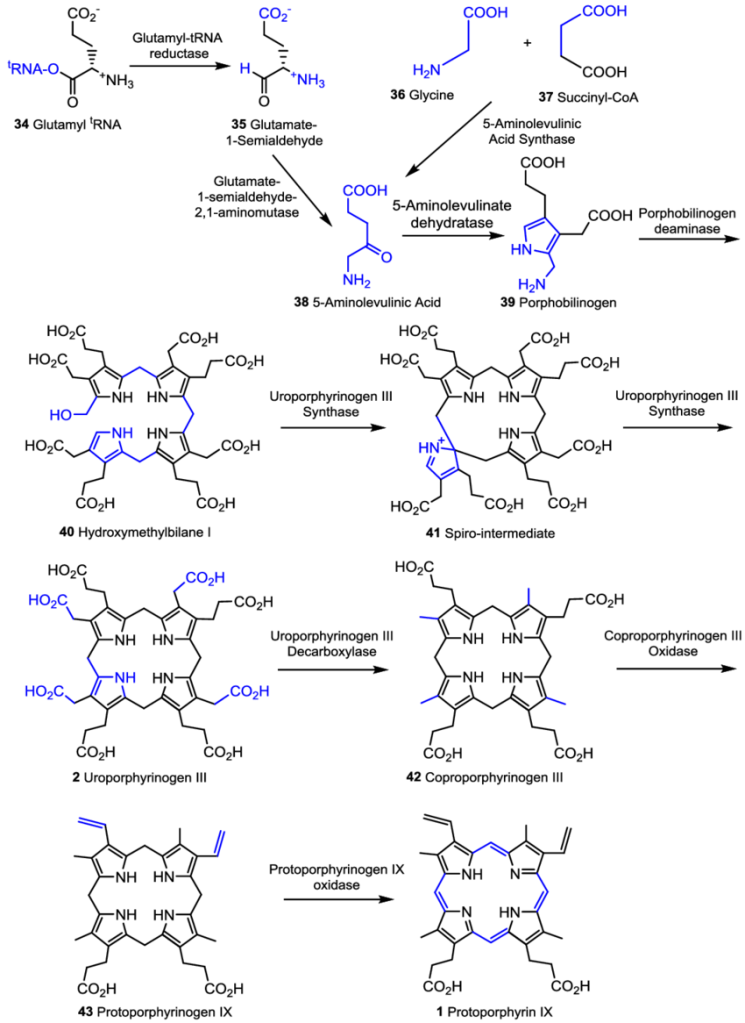
Protoporphyrin IX falls under a special type of cyclic compounds: they are macrocycles, or molecules that have a ring of twelve or more atoms. The main bulk of the molecule is called a porphine core, encircled in red in Fig. 1.
Biosynthesis begins with the formation of 5-aminolevulinic acid, which is synthesized from either glycine and succinyl-CoA from the citric acid cycle (usually in non-photosynthesizers) or from glutamyl tRNA (usually in photosynthesizers). But the process is the same for all organisms from there, shown below in Fig. 2.
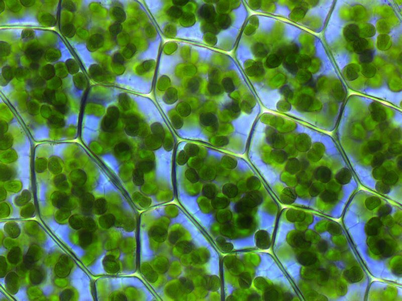
Protoporphyrin IX is a versatile molecule that is used to synthesize a variety of molecules such as heme and chlorophylls. Heme is a red pigment found in the blood and is used for oxygen delivery to body tissues. Chlorophyll (a and b) on the other hand are green pigments found in the chloroplasts of plant cells used for harvesting light energy. It’s interesting to see how both of these molecules of different color, origin, and use originate from the same substance!
Figure 3. Left to right: (a) Chloroplasts with a green chlorophyll pigment, (b) structure of chlorophyll a, (c) blood with red heme pigment (bright red – heme has oxygen bound to it, dark red – heme has no oxygen bound do it), (d) structure of heme.
Protoporphyrin IX is also used in photodynamic therapy, which is a technique to treat cancer. In this treatment, a photosensitizer – in this case, protoporphyrin IX – is made toxic by activating it with a specific wavelength of light. The toxicity of the photosensitizer can destroy cancerous and precancerous cells.
References
Battersby AR, Fookes CJR, Matcham GWJ, McDonald E. 1980. Biosynthesis of the pigments of life: Nature 285(1): 17-21.


_2%22_wafer.jpg)
#/media/File:Stockwerke_wald.png)
.jpg)
.jpeg)
.png)