Hi pure math. Yeah, YOU WON’T BE SO HAPPY NOW IF IT WEREN’T FOR YOUR APPLICATIONS.
So let’s talk about that part of math that loves continuity. I talked about it before, ehe, calculus (analysis in general), differential equations, etc. YOU WOULDN’T EXIST IF IT WEREN’T FOR PHYSICS PUSHING SOME PROBLEMS THAT REQUIRED YOU TO BE DEVELOPED IN ORDER TO SOLVE THEM. Ordinary differential equations originally described the motion of masses. Then partial differential equations came to describe wavy waves and diffusing heat. SO BE THANKFUL TO PHYSICS.
And how about that part of math that’s addicted to puzzles? Discrete math? Yeah, it wouldn’t even exist if people in the BCEs weren’t bored with puzzles, or if Euler didn’t care about that Konigsberg bridge problem, or if Turing, Lovelace, and Babbage didn’t invent the computer. Or if Hamming and von Neumann wasn’t concerned about error correction.
AND FINALLY. Probability theory. Probability theory wouldn’t be as developed today if it weren’t for physics trying to solve many-body problems or statistics trying to predict the nature of a sample size.
SO FAR the only part of pure math that I could think of that could exist without inspiration from its applications is number theory. Then again, analysis, algebra, and geometry are all used in number theory, and analysis, algebra, and geometry wouldn’t be who they are today if not for physics, computer science, etc. etc.
I COULD GO ON BUT I THINK I’VE SCITPOSTED ENOUGH TODAY, SEE PREVIOUS SCITPOSTS :)))
Haha. You probably thought calculus or differential equations was the end of your journey down, down, down the rabbit hole. Lmao no. Ok, so maybe you also acknowledged the existence of matrices and vectors in linear algebra. But then you discovered that functions are also vectors, and this property was really useful in differential equations because the derivative behaved as a linear operator and the continuous functions as a vector space. So you were like, “what a nice connection!” (or you said “what the f*** i dont like this anymore”).
But then you discover that the treatment of functions as vectors (see previous scitpost) is on a very deep level, and that functions are basically infinite dimensional vectors. And differential operators acting on functions (one-variable or multivariable) are like matrices acting on Euclidean vectors in terms of its properties. THIS IS THE TRUE LINEAR ALGEBRA GUYS.
But then you discovered there was complex-valued calculus, i.e., complex analysis. Wow, interesting extension. And then you also discovered the applications of matrices as tensors to geometric problems. Ok, not too bad, that wasn’t too hard to connect. Then you discovered that these tensors had algebraic properties that formed a group, where associativity on binary operations applied and where identity and inverse elements existed (like in rotations, where the identity is rotation by 0 degrees, and the inverse of a rotation is rotating it backwards to its original position again). So you discovered abstract algebra existed, and there were groups, rings, fields, etc.
But then you also found out there was a more rigorous way to treat calculus, i.e., mathematical analysis where you traced all your conclusions back to the fact that the real numbers are an infinitely uncountable ordered field, or its set-theoretic properties.
Ordered field? That’s abstract algebra, huh. And the set-theoretic properties could be generalized (while taking inspiration from the real numbers) to the wild field of topology, which I think is spicy set theory. Then you also discover that the set of operators over a vector space also has its own topological properties NKDJASDJASKDNAJKWDAD WHAT.
ADMIT IT. Most of you math and physics people love what you do because of all the symbols that make you feel smart when you write them down. Now don’t tell me you don’t feel satisfaction when you write
with a sign pen. I know you feel a thrill in your hands and head when you write that fancy S down. Or when you write down a differential equation like
Or some magical series with a lot of Greek letters like
Heh, I bet you also like it when you write down operators that are written down as words, like det(A), ran(f), dom(f), ker(T), dimker(T), dimran(T), and so on and so forth. Tell me, would you like mathematics if had ugly notation like
I hope not. I’m sure you would prefer
because it makes you feel smarter. I know it makes me feel smarter.
I am only beginning to realize how crucial the interpretation of functions as vectors, or elements in a vector space, is to physics. This realization had widespread effects in classical mechanics, quantum mechanics, electromagnetics,…
Interpreting functions as vectors REALLY helped in the study of Fourier analysis and calculus of variations. And those fields of mathematics are really, really, really important in the study of mechanics. Basically when you do higher physics, you’re just playing around with the properties of functions. I think. Anyway, I’m not even in graduate school yet so I can’t say, but that’s probably how it works??
Long live f such that f is a continuous function. Long live differential operators!
NO. Not the high school treatment of functions where they just find the zeroes of boring quadratic functions and the period of simple trigonometric functions. I’m talking about the vector-interpretation of functions. You got that right, functions are vectors. Not the usual real-valued vectors in 2-space or 3-space or any general n-dimensional space – you know, they one you could write as an n-tuple (x1,…,xn). I’m talking about continuous functions, which are INFINITE DIMENSIONAL VECTORS. Ok, so maybe I should define what vectors are first.
Vectors are elements in a vector space. That’s it, no comment on how many dimensions it should have, or whether or not it can be represented as as (x1,…,xn). But what exactly is a vector space?
Definition. A set V is said to be a vector space such that for any elements u, v, and w in V and for a scalar field F with a and b in F, there exists operations + and · such that
u + v is in V.
u + v = v + u
(u + v) + w = u + (v + w)
There exists an additive identity 0 such that v + 0 = 0 + v = v.
There exists an additive inverse -v such that v + (-v) = (-v) + v = 0.
a·v is in V.
a·(u + v) = a·u + a·v
(a+b)·v = a·v + b·v
a·(b·v) = (a·b)·v
There exists a multiplicative identity 1 in V such that 1·v = v.
This makes sense for vectors in Euclidean space – you know, the one with the usual point-wise addition, and real (or complex) valued scalar multiplication. But this definition also applies for functions. Let C(R) be the set of continuous functions over the real numbers R, let f, g, and h be in C(R), and let a and b be complex numbers.
f + g is also continuous therefore also in C(R)
f + g = g + f
(f + g) + h = f + (g + h)
If z(x) = 0, then f + z = z + f = f. z is the zero constant function.
f + (-f) = (-f) + f = 0
af is also a continuous function therefore also in C(R)
a(f + g) = af + ag
(a + b)f = af + bf
a(bf) = (ab)f
1f = f
See? They fulfill the properties of a vector space. So C(R) is a vector space!! BUT, there is a key difference: C(R) is infinite dimensional!
What do we mean when we say “dimension” when we talk about vector spaces? Intuitively, dimension in Euclidean space is the number of perpendicular lines or axes you can draw intersecting at a point. In 2-space, you can only draw 2 (x and y axes), and in 3-space, you can draw 3 (x, y, and z). These axes can be represented by tuples, so for two space the positive direction of these axes are represented by the unit vectors {(1,0), (0,1)} and for 3-space, {(1,0,0), (0,1,0), (0,0,1)}. These basis vectors cannot be written as a scalar multiple of the other, hence they are said to be linearly independent . All the other vectors in these spaces can be represented as a linear combination of these unit vectors (like, a scalar multiple of one of the basis vectors plus other scalar multiples of the others). For example, (2,5,3) = 2(1,0,0) + 5(0,1,0) + 3(0,0,1), (1,2,3) = (1,0,0) + 2(0,1,0) + 3(0,0,1), and generally (x,y,z) = x(1,0,0) + y(0,1,0) + z(0,0,1). This generalizes to higher dimesions 4, 5, 6, and so on.
Mathematicians define the dimension of the vector space as the minimum number of linearly independent vectors that can span the entire vector space. So what is the minimum number of linearly independent functions that can span the entire set of continuous functions over the reals. Well there isn’t any. You need infinitely many functions.
Why? Take the set of polynomials, which is a subset of the set of continuous functions over the real numbers C(R). Any polynomial can be expressed as a linear combination of {1, x, x2, x3, x4,…}. Already there is an infinite number of elements in this set. So the set of polynomials is infinite dimensional.
This can only mean that C(R) is infinite dimensional because a finite dimensional space cannot contain and infinite dimensional set. And we haven’t even considered other continuous functions: ekt, sin(nx), and cos(mx), where k, n, and m are real numbers.
Actually the study of infinite dimensional vector space is already a field of research itself, called functional analysis. That’s why functions are so cool.
I think many people would say, “it’s part of analysis!!”. After all, differential equations wouldn’t exist if functions over real numbers and their derivatives were not conceptualized. But like, woah, an introductory course in DEs wouldn’t make sense if not for our understanding of linear algebra. Functions are apparently also vectors, and derivatives are linear operators (hence they are also called differential operators).
How are functions vectors?? Let f, g, and h represent continuous functions. Well, the set of all continuous functions have an additive identity (f + 0 = f), it is closed under addition (f + g = h), they can be multiplied by a scalar (kf where k is a complex number), they have an additive inverse, etc. etc. They’re just not a finite-dimensional vector space like Euclidean space.
Derivatives are also linear operators. If D represents operation of taking the derivative of a function, then D(af + bg) = aDf + bDg for constants a and b.
Existence and uniqueness theorems regarding differential equations usually rely on concepts from real analysis (with all those wild inequalities T_T), so it also makes sense to categorize differential equations as part of analysis.
I’m so confused. We could say DEs are part of both analysis and algebra, or neither. But that’s soooo unsatisfying. I’ll just leave with the physics community’s favorite differential equations,
I mean, calculus deals with s m o o t h stuff, like the real numbers, which is infinite and uncountable. And continuous functions are s m o o t h and unbreaking, an unbreaking line or chain of points that are not isolated. They’re chads, these points are chads, with a dense number of points always surrounding them. And differentiable functions are even s m o o t h e r, because they’re continuous functions that are always cURVing.
OK WELL what about discrete math? Discrete math loves being isolated. Discrete maths isolates itself from other points (and people). Discrete maths loves to be counted, unlike the cooler real numbers that can’t be counted. Also a lot of it involves too much proof by induction, proof by contradiction, etc. etc.
Calculus, on the other hand, is a colorful girl. What other stuff does calculus like? Lol, they even capture higher dimensional shapes and regions, and even arbitrary regions. Connected arbitrary regions are also involved in calculus. You need the area of a general 2D shape? Use double integrals!! You need the volume of a general 3D region? Use triple integrals!!
Does discrete math even have these s m o o t h regions and shapes? No, it doesn’t. The closest thing it even has to shapes are graphs that represent the vertices or edges of polygons and polyhedra and higher polytopes. Well, the area and volume of these polytopes can be found using calculus… but then again there are also interesting topological concepts found in examining the vertices and edges of these shapes.
But calculus even involves Euclidean vectors in its gang, and Euclidean vectors always have direction in life. And if we have a continuous vector-valued function, it means that there is a continuum of vectors in a vector field, all flowing towards a direction. That direction is given by calculus. What a madman.
I can go on, lol. The ideas of calculus carried over to differential equations, ordinary and partial. Any function described by a differential equation is s m o o t h, like, really s m o o t h over a certain region. The myth the legend calculus introduced the idea of derivatives, and relating the function’s derivatives in a single equation like y” + t2y’ – y = sin(t) or uxx + uyy + uzz = a2utt might seem to give us more problems, but calculus knows that tackling these problems has its uses. It makes the boi physics stronger, it makes us stronger.
But then again… discrete maths makes computer science stronger. Like the graphs I mentioned are used in computational geometry and network theory.
But discrete maths loves to be counted and I don’t like counting. I like measuring.
Ok but also remember more people love discrete maths more than calculus and differential equations because of all the interesting puzzle-derived problems discrete maths has. I think people like solving puzzles, Rubik’s cube, Hanoi towers, zero sum games…
Ok fine that’s your opinion hmmmp.
ADDENDUM: Whatever, I like limits more than induction, which is why I like continuous mathematics more than discrete mathematics. Also I’m a physics major, not a computer science major. And I was never fond of puzzles so maybe that’s why I love continuous mathematics more.
We can now introduce the Schrodinger equation in its full form. As mentioned, infinite square wells do not really represent a true physical object. Physics would have a more realistic potential energy function dependent on the vector r = (x,y,z) whose magnitude is the radial distance from the origin. Thus, the general form of the equation is
Equation 18.
We now use μ instead of m for mass since the letter m will be used for letter (if you’ve taken a chemistry class, you can probably guess for what already). The second order partial derivatives of space variables (x,y,z) can be more compactly written as
Equation 19
So that the Schrodinger equation is written in its usual form:
Equation 20.
But the right hand side can be further simplified by letting
And thus equation 20 reduces to
Equation 21
It can be noticed that while En is a real number, H is an operator. This is what is called an eigenvalue equation, since multiplying the wavefunction by En serves the purpose of applying H to it.
We Can Now Discuss Atoms
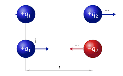
Figure 7. Charges separated by a distance
Charged particles are repelled by similarly charged particles and attracted by their oppositely charged counterparts. Their force increases if they are nearer to each other and decreases if they are farther. It’s natural to thus think that the magnitude of the potential energy increases as the distance between them decreases, because there is a greater pull or tendency for the charged particle to fall in. This relationship is described by Coloumb’s law.
Equation 22.
where k is Coulomb’s constant, q1 and q2 are the values of the charges, and r is the distance between those charges. The negative sign is only due to convention. In atoms, we have electrons with a negative charge and protons with a positive charge. In the hydrogen atom, the simplest atom, we are given an opportunity to work with a system with only one electron and one proton. We can describe the potential energy of this electron relative to its distance from the proton r with the same Coulomb’s law:
Equation 23.
where qe is the charge of the electron. We square it since the magnitude of the charge of the electron is equal to that of the proton, so essentially we’re multiplying qe by itself. Thus, Equation 19 becomes
Equation 24.
But then again we can write this in a time-independent manner since the right hand side still describes the sum of kinetic energy and potential energy.
Equation 25.
Equation 19 describes the second order space derivatives in terms of Cartesian coordinates. But we can write it in terms of spherical coordinates, that is composed of the radius from the origin, the angle of the vector counterclockwise in the xy-plane, and the angle of the vector from the z-axis.
Figure 8. Spherical coordinates.
Which can be plugged into Equation 24 to obtain
Equation 26.
Which gives an solution for the electron’s wave function around a hydrogen atom. And we will now view the wave function in spherical coordinates (r, θ, ϕ). The process of solving this is really, really long and arduous. I personally would not prefer putting it here. If you’re curious, you can opt to torture yourself by reading this article. And the solution is equally terrifying:
Equation 27.
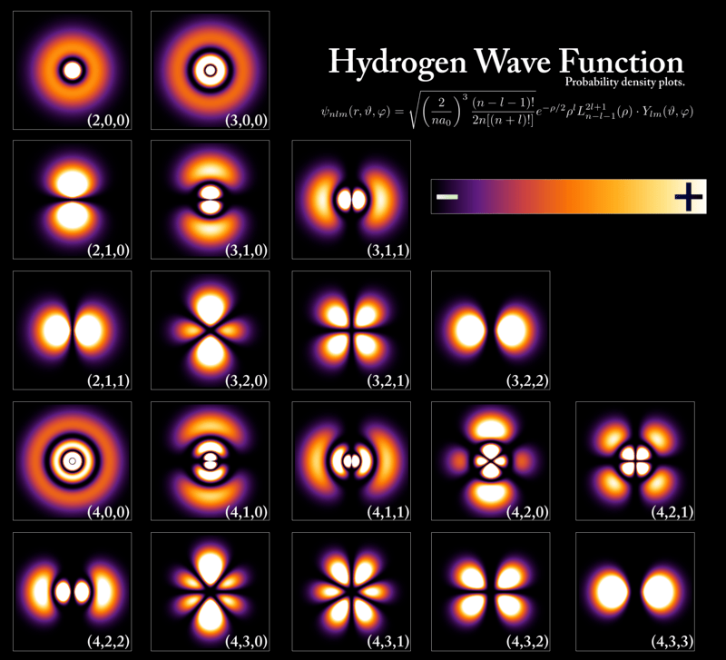
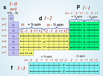
Honestly there’s no need to try and fully understand this – the only thing important to know is that r, θ, and ϕ represent variables across all of three-dimensional space and n, l, m, ħ, qe, and ε₀ are constants. But if you notice there is a subscript nlm at the left hand side. The whole of chemistry relies on Equation 27 so much that it’s almost funny – this equation describes the shapes of atomic orbitals are described. And nlm are called the quantum numbers.
First, from Equation 26 we can obtain (process not shown) the formula for the eigenvalues of energy, which is:
Equation 28.
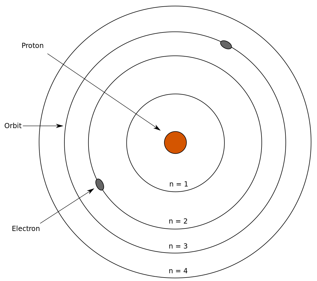
Notice that the number n, which is an integer, solely determines the energy of the wave function. In the Bohr model of the atom, n would represent the nth concentric ring away from the nucleus.
Figure 9. The Bohr model of the atom.
Thus, we call n the principal quantum number. Now that we have n, from Equation 27 in the square root term, we have (n – l – 1)! Factorials are only valid if it is a positive whole number, so we can conclude that l < n (otherwise it will be negative. Delving deeper into the equation, we can find a restriction for the values of m given that Ylm(θ, ϕ) actually represents the following:
Equation 29.
where c1 is a constant, i = √-1, and ak are terms in a series. Note that for the solution to exist, the two series must converge. The constants ak where k is any natural number is given by
Equation 29 only converges if and only if A = l(l + 1) where l is any integer such that l < n and m = -l,…,-1, 0, 1, … 1.. In other words, Equation 29 is only possible if A = l(l + 1) and m = -l,…,-1, 0, 1, … 1. The result is summarized below by Table 1 and Figure 9.
n
l
m
1
0
0
2
0
0
2
1
-1, 0, 1
3
0
0
3
1
-1, 0, 1
3
2
-2, -1, 0, 1, 2
Table 1. Possible values for n, l, m.
Figure 10. The wave functions of the hydrogen atom. The three numbers represent (n, l, m).
Here’s what’s amazing: these are the familiar atomic orbitals in chemistry. We have thus reached our goal of deriving the quantum numbers from three dimensional Schrodinger equation in spherical coordinates with a Coulombic potential (pat yourself on the back if it all made sense to you. If not, don’t give up!)
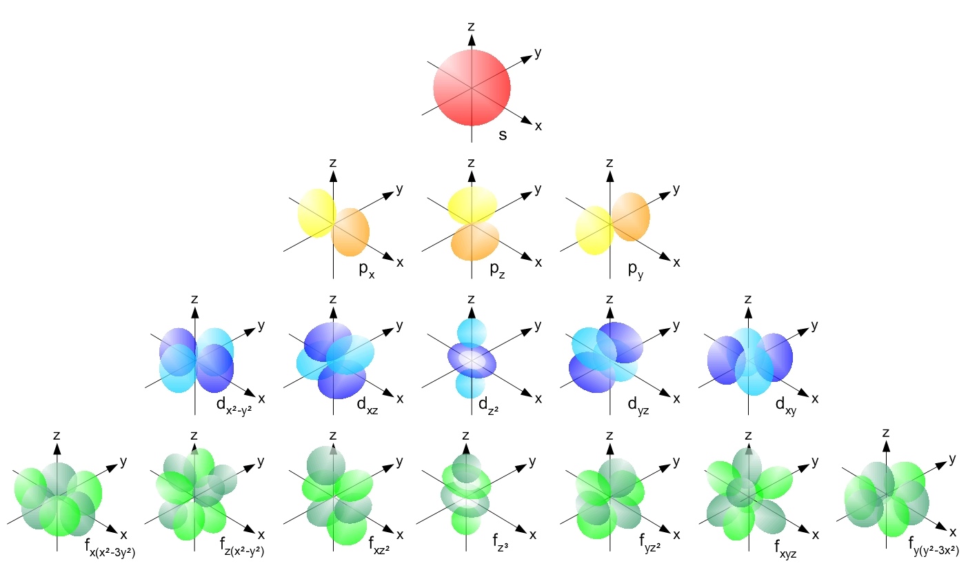
With the more familiar spdf notation from chemistry, Figure 9 closely resembles the shapes below. Remember that s represents l = 0, p represents l = 1, d represents l = 2, and f represents l = 3.
Figure 11. The spdf notation for solutions to the Schrodinger equation.
But do note that the plots in Figures 10-11 do not show the entire wave function. The wave function of any electron is spread out throughout space, and there is a change of finding a specific electron at any point in the Universe, no matter how small. The prominent shapes seen above are where the electron is to be found 90% of the time.
It’s amazing to realize that from these set of orbitals, we can start deriving the structure of the Periodic Table. Here, every row will correspond with the quantum number n, and every block that’s colored will correspond with the angular momentum number l. Every column will correspond with m which determines the orientation of the wave function around the atom.
The implications of what the Schrodinger equation predicts is basically the foundation of chemistry. Each valence electron (the outer electron) in every element corresponds with a specific wave function from Figures 10-11 – and since it is in the outer portion of the atom, that will determine how it will interact with other atoms. It will determine the element’s chemical properties, how it will bond, and what compounds it can form with other elements.
There are actually extensions of the Schrodinger equation, such as the Klein-Gordon equation and the Dirac equation. These mix in special relativity such that space and time are melded into one thing. But the consequence of that mixing is that the electron can only reach a maximum speed, which is the speed of light in the vacuum. Chemists don’t really use the Klein-Gordon or Dirac equation since the relativistic effects in chemistry are negligible.
So the Schrodinger equation up to this day remains profound. These days, computers are often used to simulate these wave functions with an arbitrary potential energy function. And for atoms with many electrons, solving the equation would practically be impossible, thus approximations such as the Hartree-Fock method are introduced. Even if it was formulated in 1925, it still remains to be a pillar of modern physics.
If you haven’t read Part 1, you should read it here before proceeding.
Infinite Square Well
In the first chapter of any quantum mechanics textbook, one would usually encounter something called the infinite square well. Basically, it is a function that describes the potential energy of any particle at location x, and in a certain length L across x, that potential energy is 0. Everywhere else, the potential energy is infinity. That is,
between 0 and L. We can interpret this as the particle being trapped in a box of length L, and it will never be able to escape. Thus, the wave function will be a wave across 0 and L, and at those edges they will be 0: Ψ(0) = 0 and Ψ(L) = 0.
Equation 5 can be recognized as a harmonic oscillator. Then the solution to this equation would be
Equation 6.
You can verify this by differentiating Ψ twice. But since Ψ(0) = 0 and Ψ(L) = 0, the value of the expression inside sin( ) must be multiples of π at 0 and L. Thus, we can say that Ψ(x) is also expressed as
Equation 7.
Since Equation 6 and Equation 7 must be the equal as they describe the same wave function, we can solve for En:
Equation 8.
Equation 8 brings us to one conclusion: since En can have varying values since n can be any integer and the rest are constants, we call En the allowed energy states dependent on n. Since En has a set of allowed values, we say that En gives the eigenvalues for the differential operator -ħ2/2m d2/dx2.
where n is any integer. The constant A is found by integrating |Ψ|2 over dx from 0 to L and equating that to 1, since |Ψ|2 represents a probability:
This process is called normalization, and the value of A could be solved for as it depends on n. But we will not tackle it here as it’s not too relevant to the discussion.
The result is thus a set of possible wave functionswith varying frequencies and wavelengths, shown in Figure 5. Although they have different properties, Equation 5 along with the fact that Ψ(0) = 0 and Ψ(L) = 0 still holds.
Figure 5. Solutions of Equation 5 dependent on the eigenvalues of En. (A) describes the classical mechanical analogy of a wave function in a box, (B) is a wave function with a wavelength of 2L with n = 1 (C) wave function with wavelength L and n = 2 (D) wave function with wavelength 2L/3 and n = 3 (E-F) are wave functions with less clear wavelengths – they’re composed of other waves. Source: https://en.wikipedia.org/wiki/Particle_in_a_box#/media/File:InfiniteSquareWellAnimation.gif
As you can see, regardless if we use the time-independent Schrodinger equation, the wave function still changes as time progresses. The time-independent wave function sort of describes the curve at a specific point in time, which regardless of when the snapshot is taken it still follows the shape of a wave.
2D Boxes and 3D Boxes
Infinite square wells aren’t actually physical objects, but they’re useful in modeling particle traps in which it would be really difficult for matter waves such as electrons to escape.
Equation 4 in Part 1 describes the Schrodinger equation in 1 dimension. But actually, we can do better by extending it to two dimensions.
Equation 9.
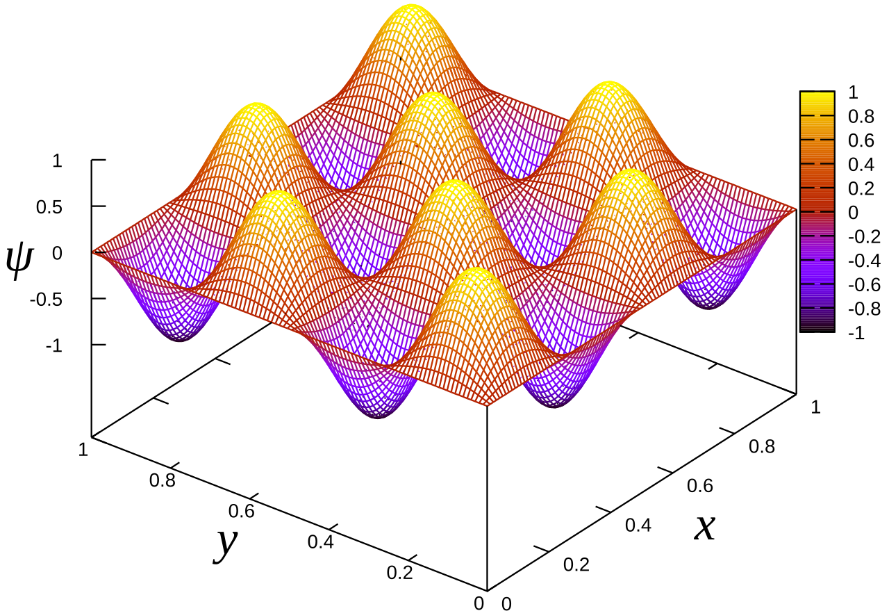
Notice that we once again use partial derivatives since the wave function Ψ(x,y) now depends on two position variables on a plane (x,y). We considered potential energy function that only depended on its position along a line, but now we allow it to depend on its position on the said plane. Well we can now formulate an infinite square well in two dimensions.
Equation 10.
where Lx is the length of the well parallel to the x axis and Ly is the length of the well parallel to the y axis. And in the places where V(x,y) = 0, this results to an equation similar to Equation 5.
Equation 11.
The solution to this is shown below along with its plot along the xy-plane where Ψ is 0 at the edges of the plane. Note however that Figure 6 only shows one particular solution.
Equation 12Figure 6. The wave function in a 2D infinite square well.
where nx and ny are arbitrary integers. The process of obtaining it is no longer shown but you can once again try it out yourself. Regardless if we set it to two dimensions, the formula given by Equation 8 still holds, but now with two terms for x and y.
Equation 13.
Solving for A in Equation 12 would require normalization involving double integrals.
We can hence further extend this to three dimensions.
Equation 14.
With potential
Equation 15.
That in the regions where V(x,y,z) = 0 reduces Equation 12 to
Equation16.
Then the solution and formula for the eigenvalues for energy are given. The equation is hard to plot, but it can be viewed in this video.
Equation 17.
Equation 18.
In summary, En gives the eigenvalues for the sum of the second order partial derivatives with respect to x, y, and z. Solving for A in Equation 17 would require normalization involving triple integrals.
In the start of any chemistry class, we’re usually shown a set of weird-looking shapes called atomic orbitals. We are given a set of rules to describe them with quantum numbers n, l, m: the quantum number n is the principal quantum number that describes how much energy it has, l determines the angular momentum magnitude and hence its shape, and m determines the orientation in 3D space. We’re only told to accept this, but we never know why.
And for good reason. Knowing why requires an understanding of partial linear differential equations and a solid grasp of quantum mechanics (everyone’s favorite popsci topic). Specifically, these atomic orbitals can be derived from what is called the Schrodinger equation.
Formulated in 1925, Erwin Schrodinger published his description of the matter wave in 1926. Up to this day, this equation is still used in modern research.
Quantum mechanics, with all its weirdness, say that these atomic orbitals represent the spaces where the electrons is most likely to be found. But why don’t electrons just stay in once place? Why don’t they just orbit in a behaved manner like Earth around the Sun?
Wave-Particle Duality
Quantum mechanics assumes that matter such as electrons are both particles and waves. Wave-like properties can be seen in the patterns in the double-slit experiment, where a stream of electrons are allowed to pass through two narrow slits. The patterns seen in Figure 1 represent the interference of wave-like electrons with each other. Figure 2 shows the mechanism with how this is possible.
This is possible because of what’s called constructive interference and destructive interference. When two waves meet and they are exactly in phase, constructive interference happens as the amplitudes get bigger. But when they are exactly out of phase, they destroy each other’s amplitudes.
But electrons also have particle-like properties. Light made out of photons – which themselves are both particles and waves at the same time – can knock off the electrons from a piece of metal when it’s given enough energy. To knock off the electrons, a collision must happen – something waves don’t do. As mentioned, when waves meet each other, they either constructively or destructively interfere with one another.
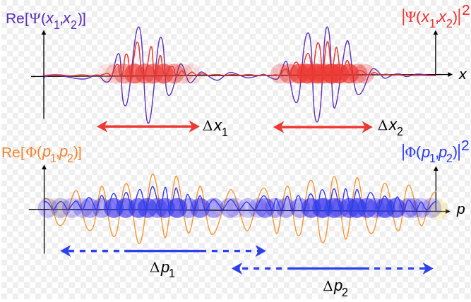
To reconcile this, physicists interpreted the wave as a sort of probability distribution of where the particle could be found. Hence, we can describe the wave as a function Ψ(x,y,z,t) – a 3D that changes over time. In particular, that probability is the square of that wave function, |Ψ|2.
This probability distribution describes where the particle is likely to be found. That’s why you’d often hear phrases such as “being at two places at the same time” – they do have chances of being found at two different position. People recognize this as the “weirdness” of QM. It would be better if we fully describe what this wave looks like.
The One-Dimensional Schrodinger Equation
In one dimension, we Schrodinger equation can be written as a function of x and t.
Equation 3.
Where i = √-1, ħ is Planck’s constant divided by 2π, m is the mass of the wave-particle (an electron, for example), and V is the potential energy dependent on the position x.
The equation looks extremely daunting at first, but actually physicists are thankful that it’s one of the few solvable partial differential equations in the sciences. We’ll describe each part bit by bit. In the right hand side of the equation,
describes the kinetic energy of the particle, and the V(x)Ψ term describes its potential energy at a given location. We can actually have any potential energy function attached to the wave function: V(r) = (1/2)r2, V(r) = r, or V(r) = k/r2 where k is any constant. The left hand side,
describes how the particle changes with respect to time. Since the right hand side of the equation involves the addition of kinetic energy and potential energy, we can interpret it as the total energy of the particle in this case. So, we may opt to drop the left hand side and instead equation it to EnΨ to obtain
Equation 4.
We no longer use the partial derivative with respective to x since this differential equation is time-independent.


