Uncovering the Schrodinger Equation [Part 2]

If you haven’t read Part 1, you should read it here before proceeding.

Infinite Square Well

In the first chapter of any quantum mechanics textbook, one would usually encounter something called the infinite square well. Basically, it is a function that describes the potential energy of any particle at location x, and in a certain length L across x, that potential energy is 0. Everywhere else, the potential energy is infinity. That is,

It can be graphically visualized in Figure 4.

Thus, Equation 4 becomes

between 0 and L. We can interpret this as the particle being trapped in a box of length L, and it will never be able to escape. Thus, the wave function will be a wave across 0 and L, and at those edges they will be 0: Ψ(0) = 0 and Ψ(L) = 0.

Equation 5 can be recognized as a harmonic oscillator. Then the solution to this equation would be

You can verify this by differentiating Ψ twice. But since Ψ(0) = 0 and Ψ(L) = 0, the value of the expression inside sin( ) must be multiples of π at 0 and L. Thus, we can say that Ψ(x) is also expressed as

Since Equation 6 and Equation 7 must be the equal as they describe the same wave function, we can solve for E_n:

Equation 8 brings us to one conclusion: since E_n can have varying values since n can be any integer and the rest are constants, we call E_n the allowed energy states dependent on n. Since E_n has a set of allowed values, we say that E_n gives the eigenvalues for the differential operator -ħ²/2m d²/dx².

where n is any integer. The constant A is found by integrating |Ψ|² over dx from 0 to L and equating that to 1, since |Ψ|² represents a probability:

This process is called normalization, and the value of A could be solved for as it depends on n. But we will not tackle it here as it’s not too relevant to the discussion.

The result is thus a set of possible wave functions with varying frequencies and wavelengths, shown in Figure 5. Although they have different properties, Equation 5 along with the fact that Ψ(0) = 0 and Ψ(L) = 0 still holds.

As you can see, regardless if we use the time-independent Schrodinger equation, the wave function still changes as time progresses. The time-independent wave function sort of describes the curve at a specific point in time, which regardless of when the snapshot is taken it still follows the shape of a wave.

2D Boxes and 3D Boxes

Infinite square wells aren’t actually physical objects, but they’re useful in modeling particle traps in which it would be really difficult for matter waves such as electrons to escape.

Equation 4 in Part 1 describes the Schrodinger equation in 1 dimension. But actually, we can do better by extending it to two dimensions.

Notice that we once again use partial derivatives since the wave function Ψ(x,y) now depends on two position variables on a plane (x,y). We considered potential energy function that only depended on its position along a line, but now we allow it to depend on its position on the said plane. Well we can now formulate an infinite square well in two dimensions.

where L_x is the length of the well parallel to the x axis and L_y is the length of the well parallel to the y axis. And in the places where V(x,y) = 0, this results to an equation similar to Equation 5.

The solution to this is shown below along with its plot along the xy-plane where Ψ is 0 at the edges of the plane. Note however that Figure 6 only shows one particular solution.

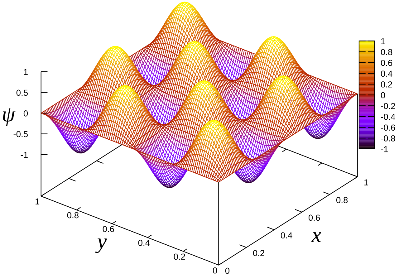
where n_x and n_y are arbitrary integers. The process of obtaining it is no longer shown but you can once again try it out yourself. Regardless if we set it to two dimensions, the formula given by Equation 8 still holds, but now with two terms for x and y.

Solving for A in Equation 12 would require normalization involving double integrals.

We can hence further extend this to three dimensions.

With potential

That in the regions where V(x,y,z) = 0 reduces Equation 12 to

Then the solution and formula for the eigenvalues for energy are given. The equation is hard to plot, but it can be viewed in this video.

In summary, E_n gives the eigenvalues for the sum of the second order partial derivatives with respect to x, y, and z. Solving for A in Equation 17 would require normalization involving triple integrals.

Proceed to Part 3