If you haven’t read Part 1, please read it here
If you haven’t read Part 2, please read it here
We can now introduce the Schrodinger equation in its full form. As mentioned, infinite square wells do not really represent a true physical object. Physics would have a more realistic potential energy function dependent on the vector r = (x,y,z) whose magnitude is the radial distance from the origin. Thus, the general form of the equation is
We now use μ instead of m for mass since the letter m will be used for letter (if you’ve taken a chemistry class, you can probably guess for what already). The second order partial derivatives of space variables (x,y,z) can be more compactly written as
So that the Schrodinger equation is written in its usual form:
But the right hand side can be further simplified by letting
And thus equation 20 reduces to
It can be noticed that while En is a real number, H is an operator. This is what is called an eigenvalue equation, since multiplying the wavefunction by En serves the purpose of applying H to it.
We Can Now Discuss Atoms
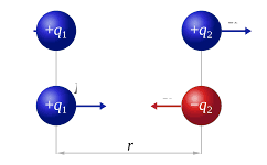
Charged particles are repelled by similarly charged particles and attracted by their oppositely charged counterparts. Their force increases if they are nearer to each other and decreases if they are farther. It’s natural to thus think that the magnitude of the potential energy increases as the distance between them decreases, because there is a greater pull or tendency for the charged particle to fall in. This relationship is described by Coloumb’s law.
where k is Coulomb’s constant, q1 and q2 are the values of the charges, and r is the distance between those charges. The negative sign is only due to convention. In atoms, we have electrons with a negative charge and protons with a positive charge. In the hydrogen atom, the simplest atom, we are given an opportunity to work with a system with only one electron and one proton. We can describe the potential energy of this electron relative to its distance from the proton r with the same Coulomb’s law:
where qe is the charge of the electron. We square it since the magnitude of the charge of the electron is equal to that of the proton, so essentially we’re multiplying qe by itself. Thus, Equation 19 becomes
But then again we can write this in a time-independent manner since the right hand side still describes the sum of kinetic energy and potential energy.
Equation 19 describes the second order space derivatives in terms of Cartesian coordinates. But we can write it in terms of spherical coordinates, that is composed of the radius from the origin, the angle of the vector counterclockwise in the xy-plane, and the angle of the vector from the z-axis.

Which can be plugged into Equation 24 to obtain
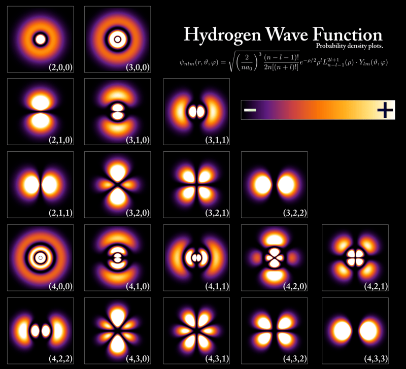
Which gives an solution for the electron’s wave function around a hydrogen atom. And we will now view the wave function in spherical coordinates (r, θ, ϕ). The process of solving this is really, really long and arduous. I personally would not prefer putting it here. If you’re curious, you can opt to torture yourself by reading this article. And the solution is equally terrifying:
Honestly there’s no need to try and fully understand this – the only thing important to know is that r, θ, and ϕ represent variables across all of three-dimensional space and n, l, m, ħ, qe, and ε₀ are constants. But if you notice there is a subscript nlm at the left hand side. The whole of chemistry relies on Equation 27 so much that it’s almost funny – this equation describes the shapes of atomic orbitals are described. And nlm are called the quantum numbers.
First, from Equation 26 we can obtain (process not shown) the formula for the eigenvalues of energy, which is:
Notice that the number n, which is an integer, solely determines the energy of the wave function. In the Bohr model of the atom, n would represent the nth concentric ring away from the nucleus.
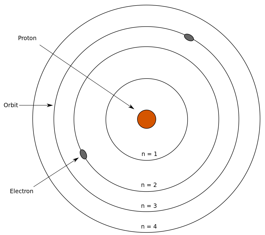
Thus, we call n the principal quantum number. Now that we have n, from Equation 27 in the square root term, we have (n – l – 1)! Factorials are only valid if it is a positive whole number, so we can conclude that l < n (otherwise it will be negative. Delving deeper into the equation, we can find a restriction for the values of m given that Ylm(θ, ϕ) actually represents the following:
where c1 is a constant, i = √-1, and ak are terms in a series. Note that for the solution to exist, the two series must converge. The constants ak where k is any natural number is given by
Equation 29 only converges if and only if A = l(l + 1) where l is any integer such that l < n and m = -l,…,-1, 0, 1, … 1.. In other words, Equation 29 is only possible if A = l(l + 1) and m = -l,…,-1, 0, 1, … 1. The result is summarized below by Table 1 and Figure 9.
| n | l | m |
| 1 | 0 | 0 |
| 2 | 0 | 0 |
| 2 | 1 | -1, 0, 1 |
| 3 | 0 | 0 |
| 3 | 1 | -1, 0, 1 |
| 3 | 2 | -2, -1, 0, 1, 2 |

Here’s what’s amazing: these are the familiar atomic orbitals in chemistry. We have thus reached our goal of deriving the quantum numbers from three dimensional Schrodinger equation in spherical coordinates with a Coulombic potential (pat yourself on the back if it all made sense to you. If not, don’t give up!)
With the more familiar spdf notation from chemistry, Figure 9 closely resembles the shapes below. Remember that s represents l = 0, p represents l = 1, d represents l = 2, and f represents l = 3.
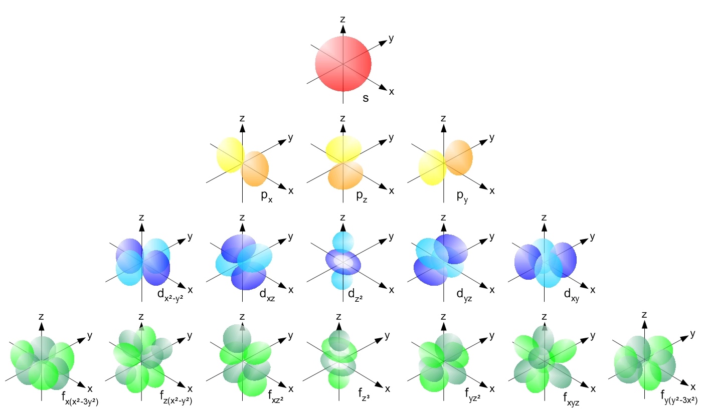
But do note that the plots in Figures 10-11 do not show the entire wave function. The wave function of any electron is spread out throughout space, and there is a change of finding a specific electron at any point in the Universe, no matter how small. The prominent shapes seen above are where the electron is to be found 90% of the time.
It’s amazing to realize that from these set of orbitals, we can start deriving the structure of the Periodic Table. Here, every row will correspond with the quantum number n, and every block that’s colored will correspond with the angular momentum number l. Every column will correspond with m which determines the orientation of the wave function around the atom.
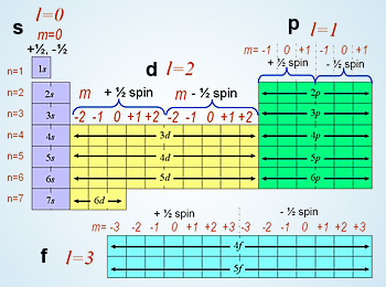
Source: https://www.simply.science/images/content/chemistry/structure_of_matter/quantum_theory/conceptmap/Quantum_numbers_Chem.html
The implications of what the Schrodinger equation predicts is basically the foundation of chemistry. Each valence electron (the outer electron) in every element corresponds with a specific wave function from Figures 10-11 – and since it is in the outer portion of the atom, that will determine how it will interact with other atoms. It will determine the element’s chemical properties, how it will bond, and what compounds it can form with other elements.
There are actually extensions of the Schrodinger equation, such as the Klein-Gordon equation and the Dirac equation. These mix in special relativity such that space and time are melded into one thing. But the consequence of that mixing is that the electron can only reach a maximum speed, which is the speed of light in the vacuum. Chemists don’t really use the Klein-Gordon or Dirac equation since the relativistic effects in chemistry are negligible.
So the Schrodinger equation up to this day remains profound. These days, computers are often used to simulate these wave functions with an arbitrary potential energy function. And for atoms with many electrons, solving the equation would practically be impossible, thus approximations such as the Hartree-Fock method are introduced. Even if it was formulated in 1925, it still remains to be a pillar of modern physics.
References
Prifysgol Aberystwyth University [Internet]. c2005. Penglais, GB: Aberystwyth University [cited 19 July 2020]. Available from: https://users.aber.ac.uk/ruw/teach/327/hatom.php.
Griffiths DJ. Introduction to Quantum Mechanics. 2015. Noida (IN-UP): Pearson India Education. 480 p.

3 thoughts on “Uncovering the Schrodinger Equation [Part 3]”